¿A dónde va Vicente?
Cuando estamos haciendo un modelo y tratamos con variables categóricas como predictoras, hay que ser muy cuidadoso. Por ejemplo hay que tener en cuenta qué pasa cuándo tenemos un nuevo nivel en el conjunto de datos a predecir que no estaba en el de entrenamiento. Por ejemplo, si estoy utilizando un algoritmo moderno tipo xgboost, y tengo como variable predictora la provincia. ¿Qué pasa si en el conjunto de entrenamiento no tengo datos de “Granada”, pero en el de predicción si?
En el xgboost por defecto las categóricas se codifican con One-Hot encoder, por lo que al no tener datos de Granada en entrenamiento a la hora de predecir la fila de Granada siempre va a tirar hacia el 0, por ejemplo, un corte en uno de los árboles podría ser Almeria = 0 para la izquierda y Almeria = 1 para la derecha. Esto es lo que suelen hacer la mayoría de las implementaciones. Pero cabe preguntarse si es la mejor solución. Otra alternativa podría ser, dado que tengo que predecir para un nivel no visto en entrenamiento, podría asignarle el valor del target que había en el nodo superior. Esta decisión plantea el problema de como sigues el proceso de partición de datos del árbol. Otra posible decisión podría ser recorrer todos los caminos posibles y promediar. En el caso anterior sería ver qué predicción acaba teniendo cuando Almería = 0 y cuando Almería = 1 y promediar. Sería una solución más justa, aunque plantea el problema de tener que recorrer más ramas.
Otra solución es en cada corte que implique a la variable categórica en cuestión, tirar hacia dónde van la mayoría de los caso “¿a dónde va Vicente? A dónde va la gente”. Esta es la solución que tiene la gente de h2o en su implementación de los Random Forest o de los Gradient Boosting. Dicen textualmente.
What happens when you try to predict on a categorical level not seen during training? Unseen categorical levels are turned into NAs, and thus follow the same behavior as an NA. If there are no NAs in the training data, then unseen categorical levels in the test data follow the majority direction (the direction with the most observations). If there are NAs in the training data, then unseen categorical levels in the test data follow the direction that is optimal for the NAs of the training data.
Ejemplo
Iniciamos h2o y cargamos datos
## Not run:
library(h2o)
h2o.init( max_mem_size = "25G")
#>  Connection successful!
#>
#> R is connected to the H2O cluster:
#>     H2O cluster uptime:         4 minutes 48 seconds
#>     H2O cluster timezone:       Europe/Madrid
#>     H2O data parsing timezone:  UTC
#>     H2O cluster version:        3.38.0.1
#>     H2O cluster version age:    1 month and 28 days
#>     H2O cluster name:           H2O_started_from_R_jose_ltm884
#>     H2O cluster total nodes:    1
#>     H2O cluster total memory:   21.82 GB
#>     H2O cluster total cores:    12
#>     H2O cluster allowed cores:  12
#>     H2O cluster healthy:        TRUE
#>     H2O Connection ip:          localhost
#>     H2O Connection port:        54321
#>     H2O Connection proxy:       NA
#>     H2O Internal Security:      FALSE
#>     R Version:                  R version 4.2.2 Patched (2022-11-10 r83330)
Importamos los datos del titanic. Ponemos como variables predictoras de la supervivencia, solo la clase y el sexo.
f <- "https://s3.amazonaws.com/h2o-public-test-data/smalldata/gbm_test/titanic.csv"
titanic <- h2o.importFile(f)
#>
  |
  |                                                                      |   0%
  |
  |======                                                                |   8%
  |
  |======================================================================| 100%

titanic['survived'] <- as.factor(titanic['survived'])
predictors <- c("pclass","sex")
response <- "survived"

# convertimos la clase a factor
titanic$pclass <- as.factor(titanic$pclass)
h2o.getTypes(titanic$pclass)
#> [[1]]
#> [1] "enum"
Partimos en train y test
splits <- h2o.splitFrame(data =  titanic, ratios = .8, seed = 1234)
train <- splits[[1]]
valid <- splits[[2]]

h2o.table(train$pclass)
#>   pclass Count
#> 1      1   260
#> 2      2   223
#> 3      3   571
#>
#> [3 rows x 2 columns]
h2o.table(train$sex)
#>      sex Count
#> 1 female   387
#> 2   male   667
#>
#> [2 rows x 2 columns]

h2o.table(valid$pclass)
#>   pclass Count
#> 1      1    63
#> 2      2    54
#> 3      3   138
#>
#> [3 rows x 2 columns]
Y ahora cambio en test para que aparezcan valores en pclass y en sex que no están en train.
valid$pclass = h2o.ifelse(valid$pclass == "3", "unknown", valid$pclass)
valid$sex    = h2o.ifelse(valid$sex == "male", "unknown", valid$sex )


h2o.table(valid$pclass)
#>    pclass Count
#> 1       1    63
#> 2       2    54
#> 3 unknown   138
#>
#> [3 rows x 2 columns]
h2o.table(valid$sex)
#>       sex Count
#> 1  female    79
#> 2 unknown   176
#>
#> [2 rows x 2 columns]
Para ver bien qué sucede con los casos en que tenemos nivel nuevo en clase y sexo nos quedamos con el siguiente conjunto de datos a predecir
test <-  valid[valid$pclass== "unknown" & valid$sex == "unknown",]
test
#>    pclass survived                          name     sex age sibsp parch ticket
#> 1 unknown        0 Abbott  Master. Eugene Joseph unknown  13     0     2    NaN
#> 2 unknown        1 Abelseth  Mr. Olaus Jorgensen unknown  25     0     0 348122
#> 3 unknown        0                Ali  Mr. Ahmed unknown  24     0     0    NaN
#> 4 unknown        0   Andersen  Mr. Albert Karvin unknown  32     0     0    NaN
#> 5 unknown        0   Andersson  Mr. Anders Johan unknown  39     1     5 347082
#> 6 unknown        0    Andreasson  Mr. Paul Edvin unknown  20     0     0 347466
#>      fare cabin embarked boat body           home.dest
#> 1 20.2500  <NA>        S  NaN  NaN East Providence  RI
#> 2  7.6500 F G63        S  NaN  NaN  Perkins County  SD
#> 3  7.0500  <NA>        S  NaN  NaN                <NA>
#> 4 22.5250  <NA>        S  NaN  260      Bergen  Norway
#> 5 31.2750  <NA>        S  NaN  NaN Sweden Winnipeg  MN
#> 6  7.8542  <NA>        S  NaN  NaN  Sweden Chicago  IL
#>
#> [99 rows x 14 columns]
Modelo xgboost
Hacemos un sólo árbol
modeloxg<-  h2o.xgboost(
  seed = 155,
  x = predictors,
  y = response,
  max_depth = 3,
  training_frame = train,
  ntrees =1
)
#>
  |
  |                                                                      |   0%
  |
  |======================================================================| 100%
Y al predecir, nos da un warning que nos dice ¡¡ojo, tengo nuevos niveles que no estaban en train!! . Aún así , no casca y devuelve una predicción
h2o.predict(modeloxg, test)
#>
  |
  |                                                                      |   0%
  |
  |======================================================================| 100%
#>   predict        p0        p1
#> 1       0 0.6016703 0.3983298
#> 2       0 0.6016703 0.3983298
#> 3       0 0.6016703 0.3983298
#> 4       0 0.6016703 0.3983298
#> 5       0 0.6016703 0.3983298
#> 6       0 0.6016703 0.3983298
#>
#> [99 rows x 3 columns]
h2o.predict_leaf_node_assignment(modeloxg, test)
#>   T1.C1
#> 1    LL
#> 2    LL
#> 3    LL
#> 4    LL
#> 5    LL
#> 6    LL
#>
#> [99 rows x 1 column]
Podemos extraer información del árbol con
arbol_ind_xg <- h2o.getModelTree(model = modeloxg, tree_number = 1)

NodesInfo <-  function(arbol_ind){
  for (i in 1:length(arbol_ind)) {
    info <-
      sprintf(
        "Node ID %s has left child node with index %s and right child node with index %s The split feature is %s. The NA direction is %s",
        arbol_ind@node_ids[i],
        arbol_ind@left_children[i],
        arbol_ind@right_children[i],
        arbol_ind@features[i],
        arbol_ind@nas[i]
      )
    print(info)
  }}

NodesInfo(arbol_ind_xg)
#> [1] "Node ID 0 has left child node with index 1 and right child node with index 2 The split feature is sex.female. The NA direction is LEFT"
#> [1] "Node ID 1 has left child node with index 3 and right child node with index 4 The split feature is pclass.1. The NA direction is LEFT"
#> [1] "Node ID 2 has left child node with index 5 and right child node with index 6 The split feature is pclass.3. The NA direction is LEFT"
#> [1] "Node ID 3 has left child node with index -1 and right child node with index -1 The split feature is NA. The NA direction is NA"
#> [1] "Node ID 4 has left child node with index -1 and right child node with index -1 The split feature is NA. The NA direction is NA"
#> [1] "Node ID 5 has left child node with index -1 and right child node with index -1 The split feature is NA. The NA direction is NA"
#> [1] "Node ID 6 has left child node with index -1 and right child node with index -1 The split feature is NA. The NA direction is NA"
Y vemos que nos da información de hacia dónde van los NA (los niveles nuevos no vistos en train) y siempre van hacia la izquierda.
Podemos pintar el árbol. Script Y vemos que los NA, siempre van hacia los 0’s.
## importo funciones , encontradas por internet, como no, para pintar el árbol
source("plot_h2o_tree.R")

titanicDataTree_XG = createDataTree(arbol_ind_xg)plotDataTree(titanicDataTree_XG, rankdir = "TB")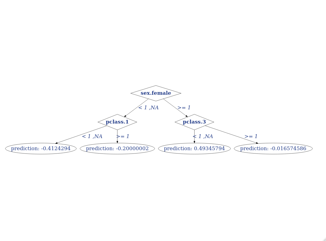
Modelo h2o.gbm
Veamos qué hace la implementación de h2o.
gbm_h2o <-  h2o.gbm(
  seed = 155,
  x = predictors,
  y = response,
  max_depth = 3,
  distribution = "bernoulli",
  training_frame = train,
  ntrees = 1
)
#>
  |
  |                                                                      |   0%
  |
  |======================================================================| 100%


h2o.predict(gbm_h2o, test)
#>
  |
  |                                                                      |   0%
  |
  |======================================================================| 100%
#>   predict        p0        p1
#> 1       0 0.6375663 0.3624337
#> 2       0 0.6375663 0.3624337
#> 3       0 0.6375663 0.3624337
#> 4       0 0.6375663 0.3624337
#> 5       0 0.6375663 0.3624337
#> 6       0 0.6375663 0.3624337
#>
#> [99 rows x 3 columns]
h2o.predict_leaf_node_assignment(gbm_h2o, test)
#>   T1.C1
#> 1   LLR
#> 2   LLR
#> 3   LLR
#> 4   LLR
#> 5   LLR
#> 6   LLR
#>
#> [99 rows x 1 column]
Y pintando lo mismo
arbol_ind <- h2o.getModelTree(model = gbm_h2o, tree_number = 1)
NodesInfo(arbol_ind )
#> [1] "Node ID 0 has left child node with index 1 and right child node with index 2 The split feature is sex. The NA direction is LEFT"
#> [1] "Node ID 1 has left child node with index 3 and right child node with index 4 The split feature is pclass. The NA direction is LEFT"
#> [1] "Node ID 2 has left child node with index 5 and right child node with index 6 The split feature is pclass. The NA direction is RIGHT"
#> [1] "Node ID 3 has left child node with index 7 and right child node with index 8 The split feature is pclass. The NA direction is RIGHT"
#> [1] "Node ID 11 has left child node with index -1 and right child node with index -1 The split feature is NA. The NA direction is NA"
#> [1] "Node ID 12 has left child node with index -1 and right child node with index -1 The split feature is NA. The NA direction is NA"
#> [1] "Node ID 6 has left child node with index 9 and right child node with index 10 The split feature is pclass. The NA direction is RIGHT"
#> [1] "Node ID 13 has left child node with index -1 and right child node with index -1 The split feature is NA. The NA direction is NA"
#> [1] "Node ID 14 has left child node with index -1 and right child node with index -1 The split feature is NA. The NA direction is NA"
#> [1] "Node ID 15 has left child node with index -1 and right child node with index -1 The split feature is NA. The NA direction is NA"
#> [1] "Node ID 16 has left child node with index -1 and right child node with index -1 The split feature is NA. The NA direction is NA"
Al pintar vemos un par de cosas curiosas, en primer lugar, h2o.gbm no ha codificado con one-hot las variables categóricas, esto permite por ejemplo que se pueden obtener reglas de corte como Izquierda:(Madrid, Barcelona, Valencia), Derecha: (resto de provincias), mientras que One Hot ese tipo de partición requiere más profundidad en el árbol. Y en segundo lugar vemos que por ejemplo los NA’s (y los nuevos niveles en test) de la variable pclass en un nodo van junto con p_class (2,3), en otro junto con p_class=1 y en otro junto p_class=3. El criterio elegido es en cada corte, los Nas y por ende los nuevos niveles no vistos en train van hacia dónde va la gente.
titanicDataTree = createDataTree(arbol_ind)
plotDataTree(titanicDataTree, rankdir = "TB")
Y nada más. hasta otra.
Nota: Los valores de prediction que saca plotDataTree no son las predicciones del modelo, sino las raw que saca ese árbol en particular. Como en los modelos de gradient boosting se va construyendo cada árbol sobre los errores del anterior, ni siquiera es la probabilidad en escala logit. He buscado en la docu de h2o pero no está claro qué es este valor. Eso sí, las ramas en el árbol están bien.