Ando viendo los vídeos de Richard McElreath , Statistical Rethinking 2022 y ciertamente me están gustando mucho. En la segunda edición de su libro hace hincapié en temas de inferencia causal. Cuenta bastante bien todo el tema de los “confounders”, “forks”, “colliders” y demás. Además lo hace simulando datos, por lo que entiende todo de forma muy sencilla. Un par de conceptos que me han llamado la atención son por ejemplo cuando dice que condicionar por una variable no significa lo mismo en un modelo de regresión al uso que en uno bayesiano, en el segundo caso significa incluir esa variable en la distribución conjunta. Esto permite por ejemplo que bajo el marco de un modelo bayesiano se pueda condicionar incluso por un “collider” cosa que los entendidos de la inferencia causal prohíben expresamente pues eso abre un camino no causal en el DAG definido.
pluralismo 1. m. Sistema por el cual se acepta o reconoce la pluralidad de doctrinas o posiciones.
y en los videos se toma dicha postura, por ejemplo, se especifica el modelo teórico utilizando los diagramas causales y el Back door criterio para ver sobre qué variables hay que condicionar o no , para ver el efecto total de X sobre Y o para estimar el efecto directo.
Nota: Este post es simplemente para entender un poco el post de Richard, el mérito es totalmente de él.
Básicamente es una situación dónde se quiere estimar el efecto que tiene sobre el número de hijos que tiene una mujer, el número de hijos que tuvo su madre. En el diagrama causal también se indica la influencia que tiene el orden de nacimiento de de la madre y de la hija.
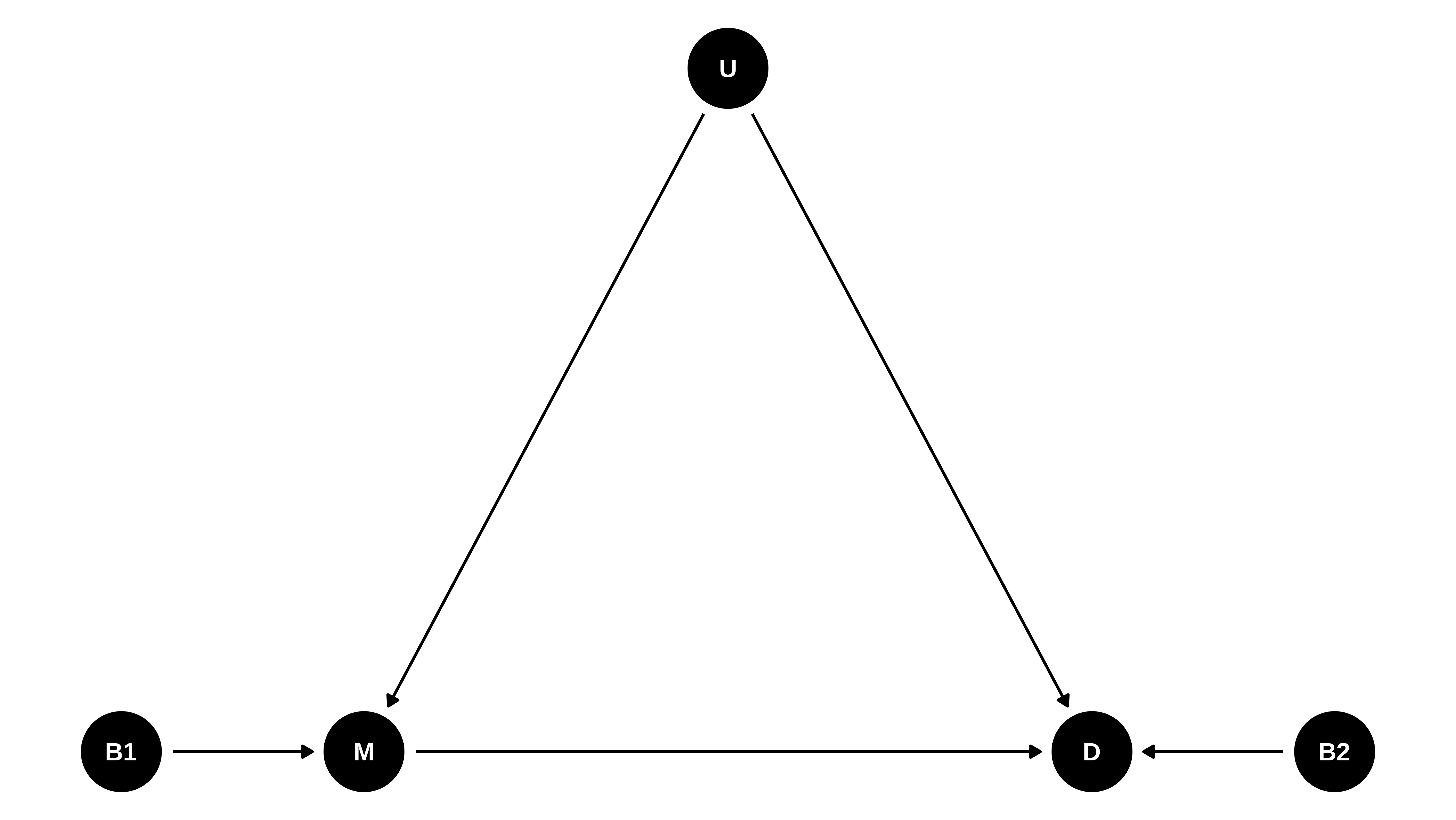
Diagrama causal:
M: Número de hijos de la madre
D: Número de hijos de la hija
B1: Orden de nacimiento de la madre
B2: Orden de nacimiento de la hija
U: Variable no medida en los datos, que pudiera ser cosas como influencia del entorno social y económico dónde viven madre e hija, que influye en las decisión del número de hijos de ambas.
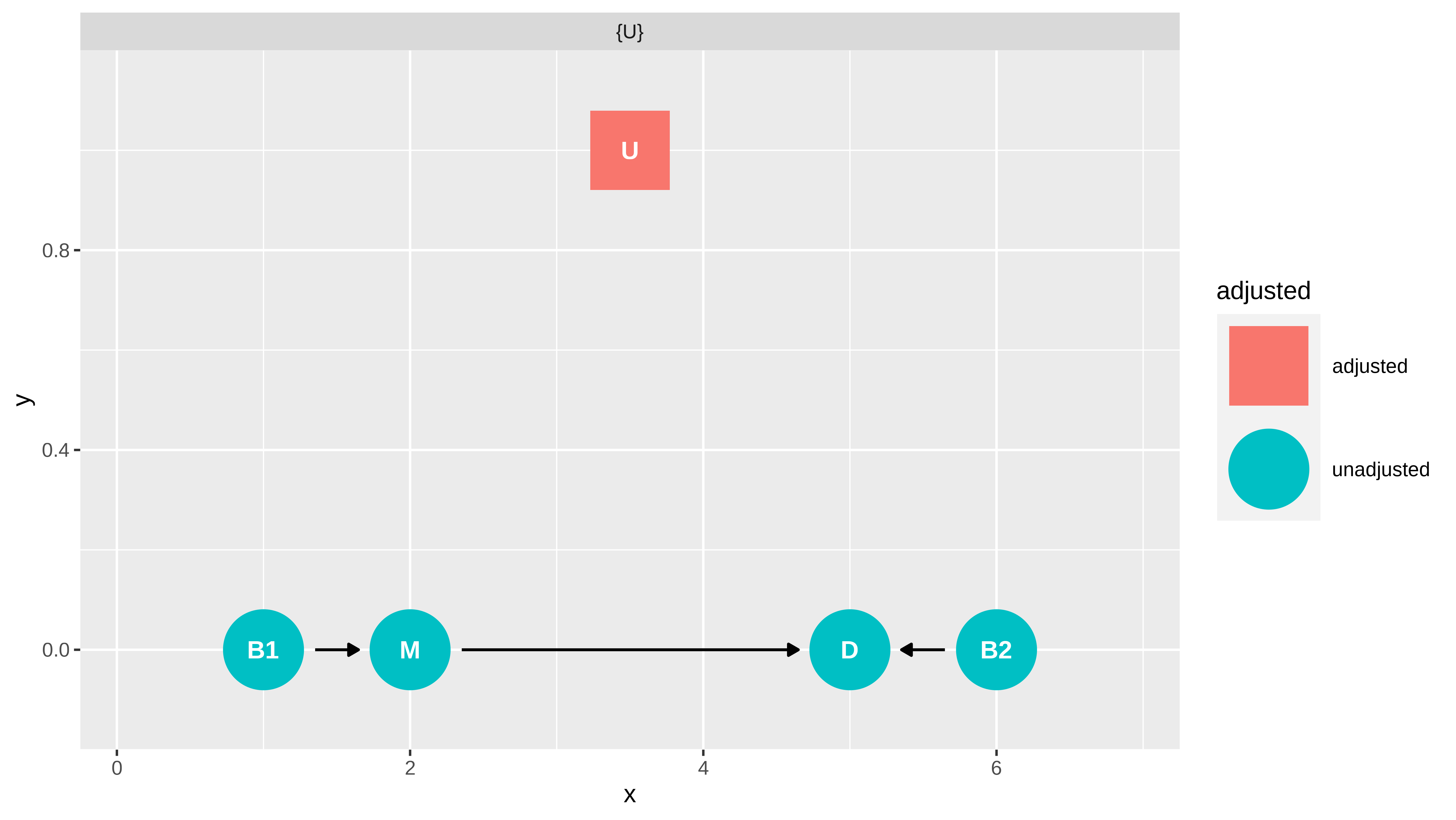
library(tidyverse)library(dagitty)library(ggdag)library(patchwork)g <-dagitty("dag{ M -> D ; B2 -> D; B1 -> M; U -> M; U -> D }")coords <-list(x =c(B1 =1, M =2, U =3.5, D =5, B2 =6),y =c(B1 =0, M =0, U =1, D =0, B2 =0))coordinates(g) <- coordsggdag(g) +theme_void()
Si queremos estimar el efecto global o el directo de M sobre D, habría que condicionar por U (siguiendo el backdoor criterio), y al ser no observable, no se puede estimar.
¿Cómo podemos “estimar” el efecto de M sobre D dado que no podemos condicionar (en el sentido clásico) sobre U? .
Richard propone lo que el llama “full luxury bayesian” que consiste en estimar a la vez todo el DAG y luego generar simulaciones usando la distribución conjunta obtenida para medir el efecto de la “intervención” y poder obtener el efecto causal.
Nótese que cuando en el DAG las relaciones se pueden expresar como modelos lineales, se puede estimar todo el DAG usando técnicas como los modelos de ecuaciones estructurales o el path analysis.
Simulación
Simulamos unos datos de forma qué vamos a conocer la “verdad” de la relaciones entre variables, que para eso simulamos.
set.seed(1908)N <-1000# número de pares, 1000 madres y 1000 hijasU <-rnorm(N,0,1) # Simulamos el confounder# orden de nacimiento y B1 <-rbinom(N,size=1,prob=0.5) # 50% de madres nacieeron en primer lugarM <-rnorm( N , 2* B1 + U )B2 <-rbinom(N,size=1,prob=0.5) # 50% son las primogénitasD <-rnorm( N , 2*B2 + U +0* M )
En esta simulación se ha forzado que el efecto del número de hijos de la madre sobre el núemro de hijos de la hija sea nulo. Por tanto sabemos que el efecto de M sobre D es 0..
Si hacemos un modelo sin condicionar, tenemos sesgo
lm(D ~ M)#> #> Call:#> lm(formula = D ~ M)#> #> Coefficients:#> (Intercept) M #> 0.7108 0.2930
Condicionando por B1 también, de hecho tenemos la situación de amplificación del sesgo
lm(D ~ M + B1)#> #> Call:#> lm(formula = D ~ M + B1)#> #> Coefficients:#> (Intercept) M B1 #> 1.0356 0.4606 -1.0441
lm(D ~ M + B1 +B2 )#> #> Call:#> lm(formula = D ~ M + B1 + B2)#> #> Coefficients:#> (Intercept) M B1 B2 #> -0.01621 0.46913 -0.91307 2.01487
lm(D ~ M + B2)#> #> Call:#> lm(formula = D ~ M + B2)#> #> Coefficients:#> (Intercept) M B2 #> -0.3204 0.3231 2.0550
En esta situación, no podemos estimar el efecto de M sobre D utilizando un solo modelo.
Una forma de estimar el efecto de M sobre D es tirar de path analysis, que en este caso se puede al ser las relaciones lineales.
Sea:
b: Efecto de B1 sobre M
m: Efecto de M sobre D
Se tiene que
\[Cov(B1, D ) = b\cdot m \cdot Var(B1)\] Y como
\[b = \dfrac{Cov(B1,M)}{Var(B1)} \]
Podemos estimar \(m\) como
\[m = \dfrac{Cov(B1,D)}{b \cdot Var(B1)} = \dfrac{Cov(B1,D)}{Cov(B1,M)} \] Y
(m_hat =cov(B1,D) /cov(B1,M))#> [1] -0.0563039
y esta estimación está menos sesgada, antes era del orden de 0.1 o 0.2 y ahora la estimación es del orden 0.01. Pero con esta estimación no tenemos información de su distribución sino sólo de esta estimación puntual. Y si las relaciones no fueran lineales no podría usarse, en cambio la siguiente aproximación si funciona
Full luxury bayes
Utilizamos la librería de Richard rethinking y también cmdstanr para expresar el modelo causal completo y ajustarlo con Stan.
Ahora estimamos el DAG completo, aquí es dónde es diferente de la aproximación causal de Pearl, de esta forma podemos “condicionar” incluso por los colliders, porque condicionar en este marco significa meter esa información dentro de la distribución conjunta.
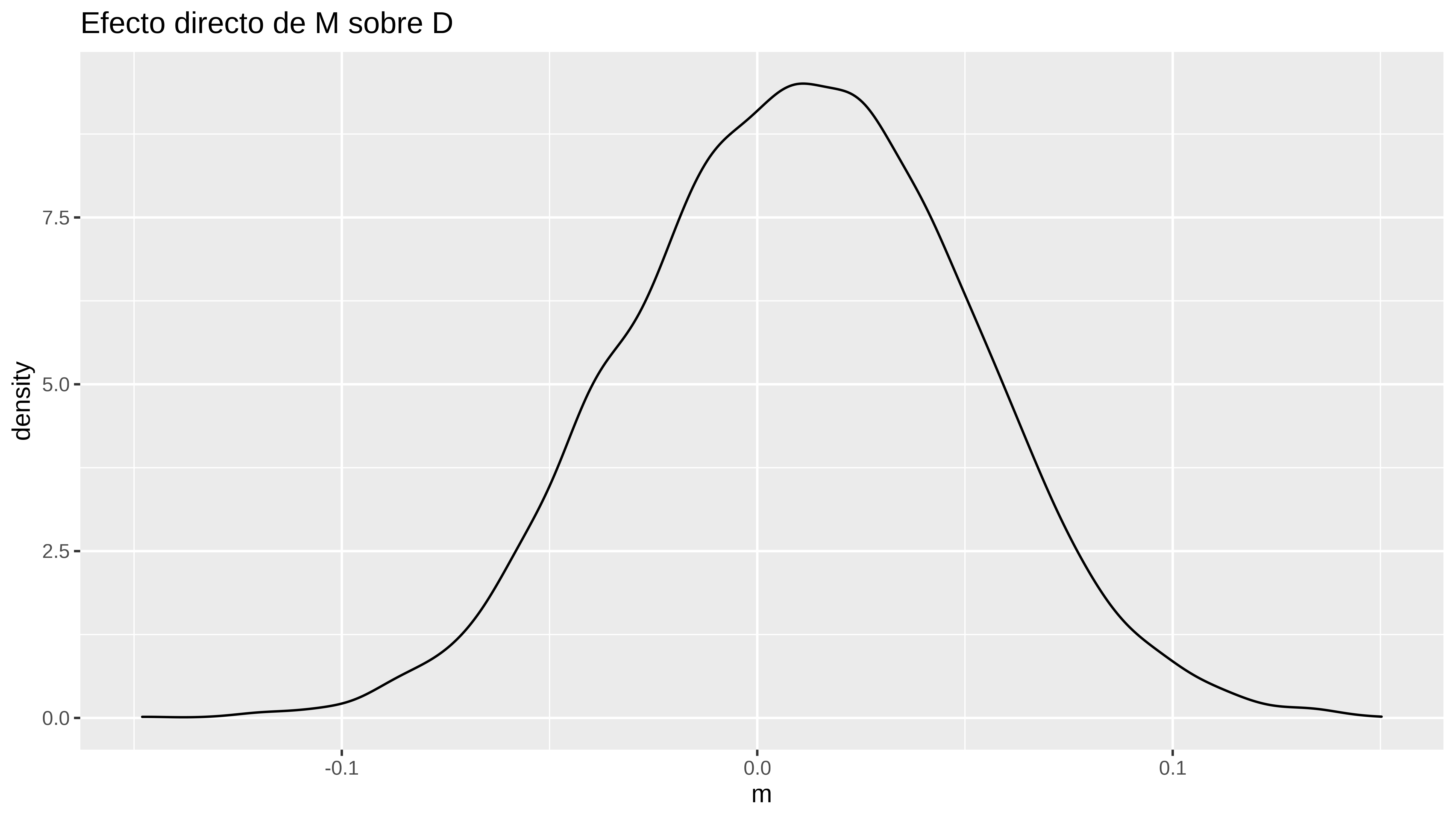
Este era el efecto que queríamos obtener y el cuál no podíamos estimar al no poder condicionar sobre U. Aquí es tan sencillo como ver su distribución a posteriori.
quantile(post$m)#> 0% 25% 50% 75% 100% #> -0.14804300 -0.01706778 0.01080760 0.03813360 0.15027000ggplot() +geom_density(aes(post$m)) +labs(title ="Efecto directo de M sobre D", x ="m")
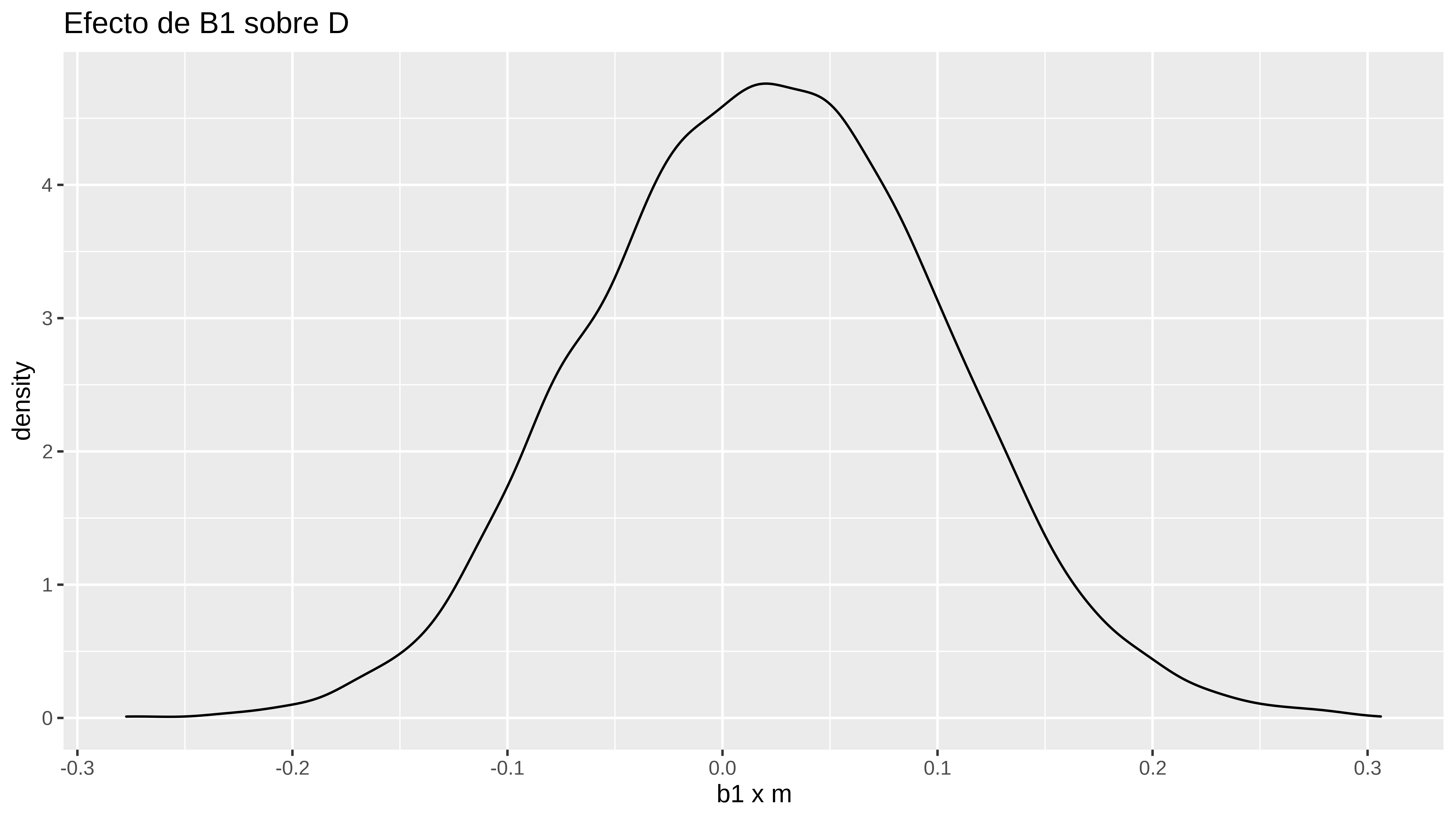
Efecto de B1 sobre D
Como ya sabíamos, al haber simulado los datos de forma que las relaciones entre las variables sean lineales, el efecto de B1 sobre D no es más que el efecto de B1 sobre M multiplicado por el efecto de M sobre D.
Utilizando la distribución a posteriori.
# Efecto de B1 sobre D quantile( with(post,b*m) )#> 0% 25% 50% 75% 100% #> -0.27728158 -0.03379382 0.02148739 0.07658919 0.30614657ggplot() +geom_density(aes(post$b * post$m))+labs(title ="Efecto de B1 sobre D", x ="b1 x m")
Efecto de B1 sobre D, simulando
Tal y como dice en su curso, el efecto causal puede ser visto como hacer una intervención supuesto cierto el modelo causal.
Simplemente utilizamos las posterioris obtenidas y vamos simulando , en primer lugar B1 = 0 y simulamos qué M se obtendría, y lo hacemos también para B1 = 1 y restamos para obtener el efecto causal, que coindice con b * m
# # B1 = 0# B1 -> MM_B1_0 <-with( post , a1 + b*0+ k*0 )# M -> DD_B1_0 <-with( post , a2 + b*0+ m*M_B1_0 + k*0 )# now same but with B1 = 1M_B1_1 <-with( post , a1 + b*1+ k*0 )D_B1_1 <-with( post , a2 + b*0+ m*M_B1_1 + k*0 )# difference to get causal effectd_D_B1 <- D_B1_1 - D_B1_0quantile(d_D_B1)#> 0% 25% 50% 75% 100% #> -0.27728158 -0.03379382 0.02148739 0.07658919 0.30614657
Pues como dice el título , ser pluralista no está tan mal, puedes usar el DAG y el backdoor criterio para entender qué variables ha de tener en cuenta para estimar tu efecto causal, y a partir de ahí podrías usar el “full luxury bayesian” en situaciones más complicadas.