set.seed(155)

N = 1000
tratamiento <- rnorm(N, 2, 1)
respuesta <- rnorm(N, 4, 1.5)

cor(tratamiento, respuesta)
[1] 0.05006728collider <- rnorm(N, 2*tratamiento + 3 * respuesta, 1.5)Continuando con temas del post anterior. Dice Pearl, con buen criterio, que si condicionas por un collider abres ese camino causal y creas una relación espuria entre las dos variables “Tratamiento” y “Respuesta” y por lo tanto si condicionas por el collider, aparece un sesgo.
Hablando estilo compadre. Si Tratamiento -> Collider y Respuesta -> Collider, si condiciono en el Collider, es decir, calculo la relación entre Tratamiento y Respuesta para cada valor de C, se introduce un sesgo.
Si \[C = 2\cdot Tratamiento + 3 \cdot respuesta\]
Si sé que C = 3, y que Tratamiento = 4 , ya hay relación entre Tratamiento y respuesta aunque sean independientes, porque ambos son causa de C.
Simulemos, que es una buena forma de ver qué pasa si condiciono por el collider, siendo el tratamiento y la respuesta independientes.
set.seed(155)
N = 1000
tratamiento <- rnorm(N, 2, 1)
respuesta <- rnorm(N, 4, 1.5)
cor(tratamiento, respuesta)[1] 0.05006728collider <- rnorm(N, 2*tratamiento + 3 * respuesta, 1.5)Si no ajusto por el collider, obtengo que no hay efecto del tratamiento , correcto
summary(lm(respuesta ~ tratamiento))
Call:
lm(formula = respuesta ~ tratamiento)

Residuals:
    Min      1Q  Median      3Q     Max
-4.7322 -1.0113 -0.0443  0.9587  6.3922

Coefficients:
            Estimate Std. Error t value Pr(>|t|)
(Intercept)  3.90287    0.10626  36.730   <2e-16 ***
tratamiento  0.07591    0.04793   1.584    0.114
---
Signif. codes:  0 '***' 0.001 '**' 0.01 '*' 0.05 '.' 0.1 ' ' 1

Residual standard error: 1.471 on 998 degrees of freedom
Multiple R-squared:  0.002507,  Adjusted R-squared:  0.001507
F-statistic: 2.508 on 1 and 998 DF,  p-value: 0.1136
Condicionando, aparece el sesgo
summary(lm(respuesta ~ tratamiento + collider))
Call:
lm(formula = respuesta ~ tratamiento + collider)

Residuals:
     Min       1Q   Median       3Q      Max
-1.59183 -0.30533  0.00423  0.30028  1.33536

Coefficients:
             Estimate Std. Error t value Pr(>|t|)
(Intercept)  0.377392   0.050478   7.476 1.67e-13 ***
tratamiento -0.599046   0.016860 -35.530  < 2e-16 ***
collider     0.300697   0.003196  94.087  < 2e-16 ***
---
Signif. codes:  0 '***' 0.001 '**' 0.01 '*' 0.05 '.' 0.1 ' ' 1

Residual standard error: 0.4683 on 997 degrees of freedom
Multiple R-squared:  0.899, Adjusted R-squared:  0.8988
F-statistic:  4439 on 2 and 997 DF,  p-value: < 2.2e-16
Retomando el ejemplo del último post, pero en vez de tener una variable de confusión no observable, tenemos un collider.
library(ggplot2)
library(dagitty)
library(ggdag)

g <- dagitty("dag{
  M -> D ;
  B2 -> D;
  B1 -> M;
  M -> C;
  D -> C
 }")


coords <-
  list(
  x = c(B1 = 1, M = 2,  C = 3.5, D = 5, B2 = 6),
  y = c(B1 = 0, M = 0, C = 1, D = 0, B2 = 0 )
)

coordinates(g) <- coords

ggdag(g) +
  theme_void()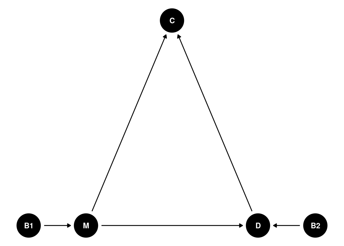
Usando la función adjustmentSets de dagitty nos dice sobre qué variables hay que condicionar si quiero el efecto causal total y directo de M sobre D, siguiendo las reglas de Pearl, ver por ejemplo (J. Pearl (2009), Causality: Models, Reasoning and Inference. Cambridge University Press.)
adjustmentSets(g, exposure = "M", outcome = "D", effect = "total" ) {}adjustmentSets(g, exposure = "M", outcome = "D", effect = "direct" ) {}Simulo unos datos dónde fuerzo a que no haya efecto causal de M a D.
set.seed(155)
N <- 1000 # número de pares, 1000 madres y 1000 hijas


 # Simulamos el collider

# orden de nacimiento y
B1 <- rbinom(N,size=1,prob=0.5)  # 50% de madres nacieeron en primer lugar
M <- rnorm( N , 2 * B1  )

B2 <- rbinom(N,size=1,prob=0.5) # 50% son las primogénitas
D <- rnorm( N , 2  * B2  + 0 * M )

# Simulamos el collider
C <- rnorm(N, 3 * M + 4*D, 2)
En grafo sería
g_sin_efecto_M_D <- dagitty("dag{
  B2 -> D;
  B1 -> M;
  M -> C;
  D -> C
 }")


coords <-
  list(
  x = c(B1 = 1, M = 2,  C = 3.5, D = 5, B2 = 6),
  y = c(B1 = 0, M = 0, C = 1, D = 0, B2 = 0 )
)

coordinates(g_sin_efecto_M_D) <- coords

ggdag(g_sin_efecto_M_D) +
  theme_void()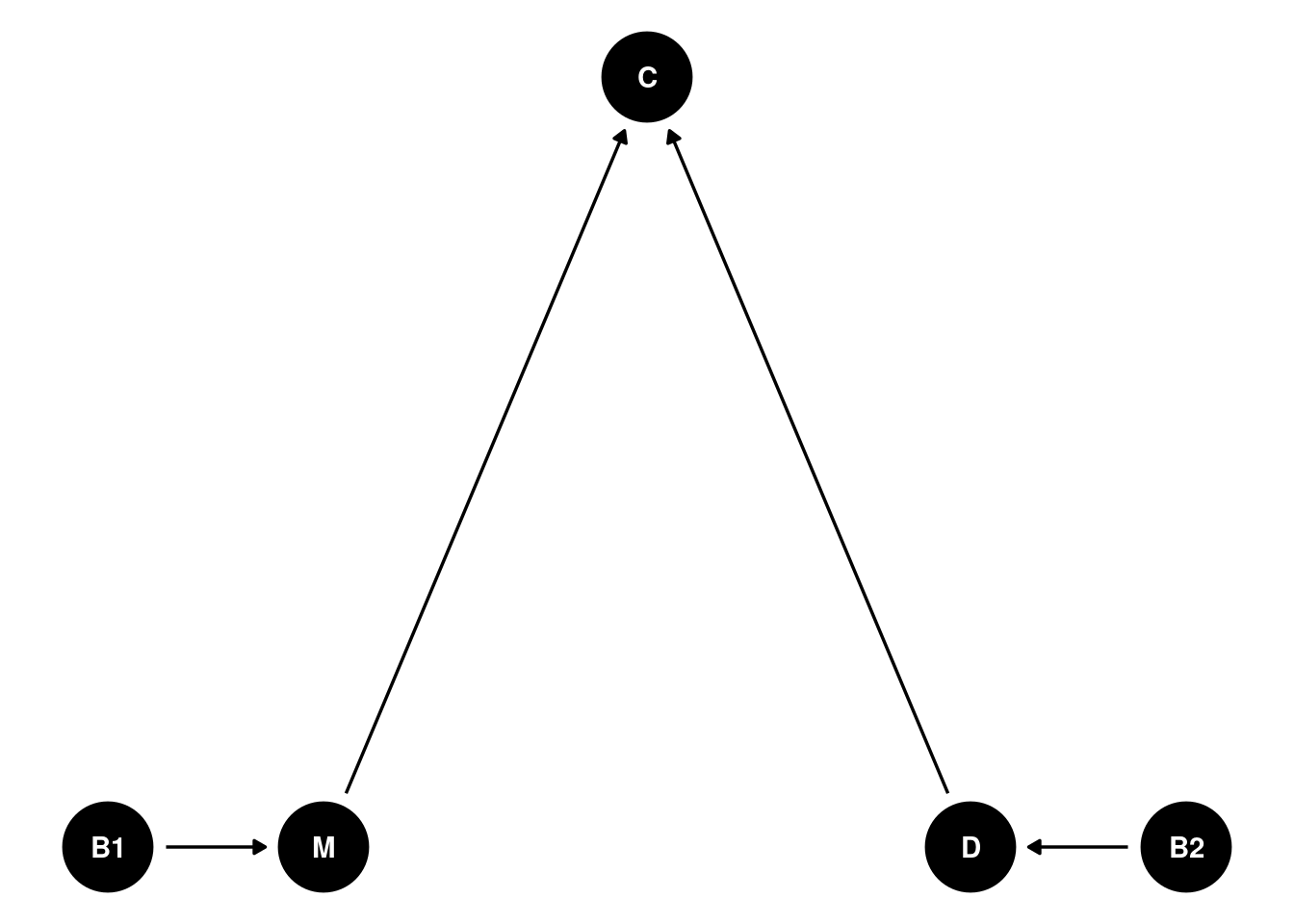
Y vemos lo de antes,
Vemos si hay efecto causal de M sobre D (uso modelos lineales por simplicidad).
El modelo correcto sería sin condicionar por el collider. Y bien, hace lo que debe, no hay efecto de M sobre D, tal y como sabemos que pasa en la realidad
summary(lm(D ~ M))
Call:
lm(formula = D ~ M)

Residuals:
    Min      1Q  Median      3Q     Max
-3.8810 -1.0553 -0.0175  1.0941  3.8417

Coefficients:
            Estimate Std. Error t value Pr(>|t|)
(Intercept)  1.02722    0.05414  18.973   <2e-16 ***
M           -0.02899    0.03207  -0.904    0.366
---
Signif. codes:  0 '***' 0.001 '**' 0.01 '*' 0.05 '.' 0.1 ' ' 1

Residual standard error: 1.398 on 998 degrees of freedom
Multiple R-squared:  0.0008181, Adjusted R-squared:  -0.0001831
F-statistic: 0.8171 on 1 and 998 DF,  p-value: 0.3662
Condicionando ahora por el collider, tenemos sesgo.
# condicionor por collider
summary(lm(D ~ M + C))
Call:
lm(formula = D ~ M + C)

Residuals:
    Min      1Q  Median      3Q     Max
-1.5621 -0.3135  0.0103  0.3344  1.5110

Coefficients:
             Estimate Std. Error t value Pr(>|t|)
(Intercept)  0.099571   0.021630   4.603 4.69e-06 ***
M           -0.654545   0.013280 -49.290  < 2e-16 ***
C            0.220029   0.002567  85.700  < 2e-16 ***
---
Signif. codes:  0 '***' 0.001 '**' 0.01 '*' 0.05 '.' 0.1 ' ' 1

Residual standard error: 0.4837 on 997 degrees of freedom
Multiple R-squared:  0.8806,    Adjusted R-squared:  0.8803
F-statistic:  3676 on 2 and 997 DF,  p-value: < 2.2e-16
# condiciono por collider y orden de nacimiento de la hija
summary(lm(D ~ M + C + B2))
Call:
lm(formula = D ~ M + C + B2)

Residuals:
    Min      1Q  Median      3Q     Max
-1.6166 -0.3133 -0.0101  0.2978  1.3493

Coefficients:
             Estimate Std. Error t value Pr(>|t|)
(Intercept) -0.021313   0.022464  -0.949    0.343
M           -0.577228   0.013905 -41.513   <2e-16 ***
C            0.194496   0.003176  61.239   <2e-16 ***
B2           0.463625   0.037877  12.240   <2e-16 ***
---
Signif. codes:  0 '***' 0.001 '**' 0.01 '*' 0.05 '.' 0.1 ' ' 1

Residual standard error: 0.4512 on 996 degrees of freedom
Multiple R-squared:  0.8962,    Adjusted R-squared:  0.8959
F-statistic:  2866 on 3 and 996 DF,  p-value: < 2.2e-16
# condiciono por collider y orden de nacimiento de la hija y de la madre
summary(lm(D ~ M + C + B2 + B1))
Call:
lm(formula = D ~ M + C + B2 + B1)

Residuals:
    Min      1Q  Median      3Q     Max
-1.6187 -0.3049 -0.0050  0.3041  1.3514

Coefficients:
             Estimate Std. Error t value Pr(>|t|)
(Intercept) -0.028298   0.024109  -1.174    0.241
M           -0.585068   0.017022 -34.371   <2e-16 ***
C            0.194286   0.003187  60.954   <2e-16 ***
B2           0.464258   0.037892  12.252   <2e-16 ***
B1           0.032672   0.040904   0.799    0.425
---
Signif. codes:  0 '***' 0.001 '**' 0.01 '*' 0.05 '.' 0.1 ' ' 1

Residual standard error: 0.4512 on 995 degrees of freedom
Multiple R-squared:  0.8963,    Adjusted R-squared:  0.8958
F-statistic:  2149 on 4 and 995 DF,  p-value: < 2.2e-16
Queda como curiosidad que si condicionas por B1 en vez de por el collider también hay sesgo, pero si condicionas solo por B2, no hay.
No todos los DAg’s son tan sencillos como el que he puesto, hay veces en los que una misma variable puede ser a la vez un collider y una variable de confusión, porque puede haber varios path causales y tenga diferente rol. En esos casos, condicionar por el collider te abre un path, y si no condicionas te abre otro. Ante esas situaciones, y suponiendo que el dag es correcto, no se podría estimar el efecto causal.
Sin embargo, condicionar en la red bayesiana no significa lo mismo que condicionar en un sólo modelo, sino que significa que introduzco la información que me proporciona el collider en la distribución conjunta y que me obtenga la posteriori.
Al estimar el DAG completo, usando Stan por ejemplo, se estima tanto el modelo para M, como para D de forma conjunta.
Formulamos el modelo usando la librería rethinking y lo ajustamos usando la función ulam que por debajo llama a Stan
library(cmdstanr)
library(rethinking)
set_cmdstan_path("~/Descargas/cmdstan/")
dat <- list(
N = N,
M = M,
D = D,
B1 = B1,
B2 = B2,
C = C
)
set.seed(155)
flbi <- ulam(
alist(
# mom model
M ~ normal( mu , sigma ),
mu <- a1 + b*B1 ,
# daughter model
D ~ normal( nu , tau ),
nu <- a2 + b*B2 + m*M ,
# B1 and B2
B1 ~ bernoulli(p),
B2 ~ bernoulli(p),
# priors
c(a1,a2,b,m) ~ normal( 0 , 0.5 ),
c(k,sigma,tau) ~ exponential( 1 ),
p ~ beta(2,2)
), data=dat , chains=4 , cores=4 , warmup = 500, iter=2500 , cmdstan=TRUE )Warning in '/tmp/Rtmpsdysi4/model-8eef3881083c.stan', line 6, column 4: Declaration
of arrays by placing brackets after a variable name is deprecated and
will be removed in Stan 2.32.0. Instead use the array keyword before the
type. This can be changed automatically using the auto-format flag to
stanc
Warning in '/tmp/Rtmpsdysi4/model-8eef3881083c.stan', line 7, column 4: Declaration
of arrays by placing brackets after a variable name is deprecated and
will be removed in Stan 2.32.0. Instead use the array keyword before the
type. This can be changed automatically using the auto-format flag to
stancRunning MCMC with 4 parallel chains, with 1 thread(s) per chain...
Chain 1 Iteration: 1 / 2500 [ 0%] (Warmup)
Chain 2 Iteration: 1 / 2500 [ 0%] (Warmup) Chain 2 Informational Message: The current Metropolis proposal is about to be rejected because of the following issue:Chain 2 Exception: normal_lpdf: Scale parameter is 0, but must be positive! (in '/tmp/Rtmpsdysi4/model-8eef3881083c.stan', line 39, column 4 to column 29)Chain 2 If this warning occurs sporadically, such as for highly constrained variable types like covariance matrices, then the sampler is fine,Chain 2 but if this warning occurs often then your model may be either severely ill-conditioned or misspecified.Chain 2 Chain 3 Iteration: 1 / 2500 [ 0%] (Warmup) Chain 3 Informational Message: The current Metropolis proposal is about to be rejected because of the following issue:Chain 3 Exception: normal_lpdf: Scale parameter is 0, but must be positive! (in '/tmp/Rtmpsdysi4/model-8eef3881083c.stan', line 39, column 4 to column 29)Chain 3 If this warning occurs sporadically, such as for highly constrained variable types like covariance matrices, then the sampler is fine,Chain 3 but if this warning occurs often then your model may be either severely ill-conditioned or misspecified.Chain 3 Chain 4 Iteration: 1 / 2500 [ 0%] (Warmup) Chain 4 Informational Message: The current Metropolis proposal is about to be rejected because of the following issue:Chain 4 Exception: normal_lpdf: Scale parameter is 0, but must be positive! (in '/tmp/Rtmpsdysi4/model-8eef3881083c.stan', line 35, column 4 to column 27)Chain 4 If this warning occurs sporadically, such as for highly constrained variable types like covariance matrices, then the sampler is fine,Chain 4 but if this warning occurs often then your model may be either severely ill-conditioned or misspecified.Chain 4 Chain 1 Iteration: 100 / 2500 [ 4%] (Warmup)
Chain 2 Iteration: 100 / 2500 [ 4%] (Warmup)
Chain 4 Iteration: 100 / 2500 [ 4%] (Warmup)
Chain 1 Iteration: 200 / 2500 [ 8%] (Warmup)
Chain 2 Iteration: 200 / 2500 [ 8%] (Warmup)
Chain 3 Iteration: 100 / 2500 [ 4%] (Warmup)
Chain 4 Iteration: 200 / 2500 [ 8%] (Warmup)
Chain 1 Iteration: 300 / 2500 [ 12%] (Warmup)
Chain 3 Iteration: 200 / 2500 [ 8%] (Warmup)
Chain 4 Iteration: 300 / 2500 [ 12%] (Warmup)
Chain 1 Iteration: 400 / 2500 [ 16%] (Warmup)
Chain 2 Iteration: 300 / 2500 [ 12%] (Warmup)
Chain 3 Iteration: 300 / 2500 [ 12%] (Warmup)
Chain 4 Iteration: 400 / 2500 [ 16%] (Warmup)
Chain 1 Iteration: 500 / 2500 [ 20%] (Warmup)
Chain 1 Iteration: 501 / 2500 [ 20%] (Sampling)
Chain 2 Iteration: 400 / 2500 [ 16%] (Warmup)
Chain 3 Iteration: 400 / 2500 [ 16%] (Warmup)
Chain 4 Iteration: 500 / 2500 [ 20%] (Warmup)
Chain 4 Iteration: 501 / 2500 [ 20%] (Sampling)
Chain 4 Iteration: 600 / 2500 [ 24%] (Sampling)
Chain 1 Iteration: 600 / 2500 [ 24%] (Sampling)
Chain 2 Iteration: 500 / 2500 [ 20%] (Warmup)
Chain 2 Iteration: 501 / 2500 [ 20%] (Sampling)
Chain 3 Iteration: 500 / 2500 [ 20%] (Warmup)
Chain 3 Iteration: 501 / 2500 [ 20%] (Sampling)
Chain 3 Iteration: 600 / 2500 [ 24%] (Sampling)
Chain 4 Iteration: 700 / 2500 [ 28%] (Sampling)
Chain 1 Iteration: 700 / 2500 [ 28%] (Sampling)
Chain 1 Iteration: 800 / 2500 [ 32%] (Sampling)
Chain 2 Iteration: 600 / 2500 [ 24%] (Sampling)
Chain 3 Iteration: 700 / 2500 [ 28%] (Sampling)
Chain 4 Iteration: 800 / 2500 [ 32%] (Sampling)
Chain 1 Iteration: 900 / 2500 [ 36%] (Sampling)
Chain 2 Iteration: 700 / 2500 [ 28%] (Sampling)
Chain 2 Iteration: 800 / 2500 [ 32%] (Sampling)
Chain 3 Iteration: 800 / 2500 [ 32%] (Sampling)
Chain 4 Iteration: 900 / 2500 [ 36%] (Sampling)
Chain 1 Iteration: 1000 / 2500 [ 40%] (Sampling)
Chain 2 Iteration: 900 / 2500 [ 36%] (Sampling)
Chain 3 Iteration: 900 / 2500 [ 36%] (Sampling)
Chain 4 Iteration: 1000 / 2500 [ 40%] (Sampling)
Chain 1 Iteration: 1100 / 2500 [ 44%] (Sampling)
Chain 1 Iteration: 1200 / 2500 [ 48%] (Sampling)
Chain 2 Iteration: 1000 / 2500 [ 40%] (Sampling)
Chain 3 Iteration: 1000 / 2500 [ 40%] (Sampling)
Chain 3 Iteration: 1100 / 2500 [ 44%] (Sampling)
Chain 4 Iteration: 1100 / 2500 [ 44%] (Sampling)
Chain 1 Iteration: 1300 / 2500 [ 52%] (Sampling)
Chain 2 Iteration: 1100 / 2500 [ 44%] (Sampling)
Chain 3 Iteration: 1200 / 2500 [ 48%] (Sampling)
Chain 4 Iteration: 1200 / 2500 [ 48%] (Sampling)
Chain 1 Iteration: 1400 / 2500 [ 56%] (Sampling)
Chain 1 Iteration: 1500 / 2500 [ 60%] (Sampling)
Chain 2 Iteration: 1200 / 2500 [ 48%] (Sampling)
Chain 3 Iteration: 1300 / 2500 [ 52%] (Sampling)
Chain 4 Iteration: 1300 / 2500 [ 52%] (Sampling)
Chain 1 Iteration: 1600 / 2500 [ 64%] (Sampling)
Chain 2 Iteration: 1300 / 2500 [ 52%] (Sampling)
Chain 3 Iteration: 1400 / 2500 [ 56%] (Sampling)
Chain 3 Iteration: 1500 / 2500 [ 60%] (Sampling)
Chain 4 Iteration: 1400 / 2500 [ 56%] (Sampling)
Chain 1 Iteration: 1700 / 2500 [ 68%] (Sampling)
Chain 2 Iteration: 1400 / 2500 [ 56%] (Sampling)
Chain 3 Iteration: 1600 / 2500 [ 64%] (Sampling)
Chain 4 Iteration: 1500 / 2500 [ 60%] (Sampling)
Chain 1 Iteration: 1800 / 2500 [ 72%] (Sampling)
Chain 2 Iteration: 1500 / 2500 [ 60%] (Sampling)
Chain 3 Iteration: 1700 / 2500 [ 68%] (Sampling)
Chain 4 Iteration: 1600 / 2500 [ 64%] (Sampling)
Chain 1 Iteration: 1900 / 2500 [ 76%] (Sampling)
Chain 1 Iteration: 2000 / 2500 [ 80%] (Sampling)
Chain 2 Iteration: 1600 / 2500 [ 64%] (Sampling)
Chain 3 Iteration: 1800 / 2500 [ 72%] (Sampling)
Chain 4 Iteration: 1700 / 2500 [ 68%] (Sampling)
Chain 4 Iteration: 1800 / 2500 [ 72%] (Sampling)
Chain 1 Iteration: 2100 / 2500 [ 84%] (Sampling)
Chain 2 Iteration: 1700 / 2500 [ 68%] (Sampling)
Chain 3 Iteration: 1900 / 2500 [ 76%] (Sampling)
Chain 3 Iteration: 2000 / 2500 [ 80%] (Sampling)
Chain 4 Iteration: 1900 / 2500 [ 76%] (Sampling)
Chain 1 Iteration: 2200 / 2500 [ 88%] (Sampling)
Chain 1 Iteration: 2300 / 2500 [ 92%] (Sampling)
Chain 2 Iteration: 1800 / 2500 [ 72%] (Sampling)
Chain 3 Iteration: 2100 / 2500 [ 84%] (Sampling)
Chain 4 Iteration: 2000 / 2500 [ 80%] (Sampling)
Chain 1 Iteration: 2400 / 2500 [ 96%] (Sampling)
Chain 2 Iteration: 1900 / 2500 [ 76%] (Sampling)
Chain 2 Iteration: 2000 / 2500 [ 80%] (Sampling)
Chain 3 Iteration: 2200 / 2500 [ 88%] (Sampling)
Chain 4 Iteration: 2100 / 2500 [ 84%] (Sampling)
Chain 1 Iteration: 2500 / 2500 [100%] (Sampling)
Chain 2 Iteration: 2100 / 2500 [ 84%] (Sampling)
Chain 3 Iteration: 2300 / 2500 [ 92%] (Sampling)
Chain 3 Iteration: 2400 / 2500 [ 96%] (Sampling)
Chain 4 Iteration: 2200 / 2500 [ 88%] (Sampling)
Chain 1 finished in 2.2 seconds.
Chain 2 Iteration: 2200 / 2500 [ 88%] (Sampling)
Chain 3 Iteration: 2500 / 2500 [100%] (Sampling)
Chain 4 Iteration: 2300 / 2500 [ 92%] (Sampling)
Chain 3 finished in 2.3 seconds.
Chain 2 Iteration: 2300 / 2500 [ 92%] (Sampling)
Chain 4 Iteration: 2400 / 2500 [ 96%] (Sampling)
Chain 4 Iteration: 2500 / 2500 [100%] (Sampling)
Chain 4 finished in 2.4 seconds.
Chain 2 Iteration: 2400 / 2500 [ 96%] (Sampling)
Chain 2 Iteration: 2500 / 2500 [100%] (Sampling)
Chain 2 finished in 2.5 seconds.
All 4 chains finished successfully.
Mean chain execution time: 2.4 seconds.
Total execution time: 2.6 seconds.Vemos los parámetros estimados y sus intervalos de credibilidad y extraemos la posteriori
precis(flbi) mean sd 5.5% 94.5% n_eff Rhat4
m -0.008692293 0.02258036 -0.044472871 0.02734239 6673.459 1.0005257
b 1.961391786 0.04356684 1.891207250 2.03241110 5380.781 0.9998034
a2 0.059745778 0.04370034 -0.009909845 0.12931849 5500.657 1.0000543
a1 0.026656585 0.03702030 -0.032118024 0.08601562 6410.710 0.9997482
tau 0.984889552 0.02213892 0.949803835 1.02046055 7752.122 1.0000469
sigma 0.967785086 0.02155725 0.933665955 1.00275110 8907.866 1.0001535
k 0.998568923 1.01036660 0.056543283 2.88207040 9005.060 1.0000657
p 0.482860133 0.01114257 0.465039000 0.50049459 8082.865 1.0000378post <- extract.samples(flbi)Pintamos la distribución a posteriori del efecto y cómo ya sabíamos, al no condicionar por el collider, se estima sin sesgo que no hay efecto causal de M a D.
plot(bayestestR::hdi(post$m, ci = c( 0.80, 0.95))) +
  labs(title = "Estimación sin collider")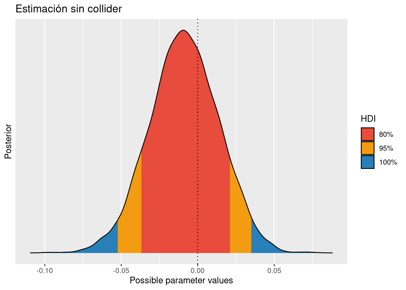
Ya sabemos que no es necesario de hecho condicionar por el collider, más aún, que hacerlo induce un sesgo en la estimación del efecto, ¿pero qué pasa si estimamos el dag al completo?
set.seed(155)

flbi_collider <- ulam(
  alist(
    # mom model
    M ~ normal( mu , sigma ),
    mu <- a1 + b*B1 ,
    # daughter model
    D ~ normal( nu , tau ),
    nu <- a2 + b*B2 + m*M ,
    # B1 and B2
    B1 ~ bernoulli(p),
    B2 ~ bernoulli(p),

    # Collider

     C ~ normal( cmu , csigma ),
     cmu <- a3 + cm * M  + cd * D,

    # priors
    c(a1,a2,a3,b,m, cm, cd) ~ normal( 0 , 0.5 ),
    c(sigma,tau, csigma) ~ exponential( 1 ),
    p ~ beta(2,2)
  ), data=dat , chains=4 , cores=4 , warmup = 500, iter=2500 , cmdstan=TRUE )
Warning in '/tmp/Rtmpsdysi4/model-8eef4e4ce260.stan', line 3, column 4: Declaration
of arrays by placing brackets after a variable name is deprecated and
will be removed in Stan 2.32.0. Instead use the array keyword before the
type. This can be changed automatically using the auto-format flag to
stanc
Warning in '/tmp/Rtmpsdysi4/model-8eef4e4ce260.stan', line 4, column 4: Declaration
of arrays by placing brackets after a variable name is deprecated and
will be removed in Stan 2.32.0. Instead use the array keyword before the
type. This can be changed automatically using the auto-format flag to
stancRunning MCMC with 4 parallel chains, with 1 thread(s) per chain...
Chain 1 Iteration: 1 / 2500 [ 0%] (Warmup)
Chain 2 Iteration: 1 / 2500 [ 0%] (Warmup)
Chain 3 Iteration: 1 / 2500 [ 0%] (Warmup)
Chain 4 Iteration: 1 / 2500 [ 0%] (Warmup)
Chain 1 Iteration: 100 / 2500 [ 4%] (Warmup)
Chain 2 Iteration: 100 / 2500 [ 4%] (Warmup)
Chain 3 Iteration: 100 / 2500 [ 4%] (Warmup)
Chain 4 Iteration: 100 / 2500 [ 4%] (Warmup)
Chain 1 Iteration: 200 / 2500 [ 8%] (Warmup)
Chain 2 Iteration: 200 / 2500 [ 8%] (Warmup)
Chain 3 Iteration: 200 / 2500 [ 8%] (Warmup)
Chain 4 Iteration: 200 / 2500 [ 8%] (Warmup)
Chain 1 Iteration: 300 / 2500 [ 12%] (Warmup)
Chain 2 Iteration: 300 / 2500 [ 12%] (Warmup)
Chain 3 Iteration: 300 / 2500 [ 12%] (Warmup)
Chain 4 Iteration: 300 / 2500 [ 12%] (Warmup)
Chain 1 Iteration: 400 / 2500 [ 16%] (Warmup)
Chain 2 Iteration: 400 / 2500 [ 16%] (Warmup)
Chain 3 Iteration: 400 / 2500 [ 16%] (Warmup)
Chain 4 Iteration: 400 / 2500 [ 16%] (Warmup)
Chain 3 Iteration: 500 / 2500 [ 20%] (Warmup)
Chain 3 Iteration: 501 / 2500 [ 20%] (Sampling)
Chain 1 Iteration: 500 / 2500 [ 20%] (Warmup)
Chain 1 Iteration: 501 / 2500 [ 20%] (Sampling)
Chain 2 Iteration: 500 / 2500 [ 20%] (Warmup)
Chain 2 Iteration: 501 / 2500 [ 20%] (Sampling)
Chain 4 Iteration: 500 / 2500 [ 20%] (Warmup)
Chain 4 Iteration: 501 / 2500 [ 20%] (Sampling)
Chain 3 Iteration: 600 / 2500 [ 24%] (Sampling)
Chain 4 Iteration: 600 / 2500 [ 24%] (Sampling)
Chain 1 Iteration: 600 / 2500 [ 24%] (Sampling)
Chain 2 Iteration: 600 / 2500 [ 24%] (Sampling)
Chain 1 Iteration: 700 / 2500 [ 28%] (Sampling)
Chain 3 Iteration: 700 / 2500 [ 28%] (Sampling)
Chain 4 Iteration: 700 / 2500 [ 28%] (Sampling)
Chain 2 Iteration: 700 / 2500 [ 28%] (Sampling)
Chain 1 Iteration: 800 / 2500 [ 32%] (Sampling)
Chain 2 Iteration: 800 / 2500 [ 32%] (Sampling)
Chain 3 Iteration: 800 / 2500 [ 32%] (Sampling)
Chain 4 Iteration: 800 / 2500 [ 32%] (Sampling)
Chain 1 Iteration: 900 / 2500 [ 36%] (Sampling)
Chain 2 Iteration: 900 / 2500 [ 36%] (Sampling)
Chain 3 Iteration: 900 / 2500 [ 36%] (Sampling)
Chain 4 Iteration: 900 / 2500 [ 36%] (Sampling)
Chain 1 Iteration: 1000 / 2500 [ 40%] (Sampling)
Chain 3 Iteration: 1000 / 2500 [ 40%] (Sampling)
Chain 4 Iteration: 1000 / 2500 [ 40%] (Sampling)
Chain 2 Iteration: 1000 / 2500 [ 40%] (Sampling)
Chain 1 Iteration: 1100 / 2500 [ 44%] (Sampling)
Chain 3 Iteration: 1100 / 2500 [ 44%] (Sampling)
Chain 4 Iteration: 1100 / 2500 [ 44%] (Sampling)
Chain 2 Iteration: 1100 / 2500 [ 44%] (Sampling)
Chain 1 Iteration: 1200 / 2500 [ 48%] (Sampling)
Chain 2 Iteration: 1200 / 2500 [ 48%] (Sampling)
Chain 3 Iteration: 1200 / 2500 [ 48%] (Sampling)
Chain 4 Iteration: 1200 / 2500 [ 48%] (Sampling)
Chain 4 Iteration: 1300 / 2500 [ 52%] (Sampling)
Chain 1 Iteration: 1300 / 2500 [ 52%] (Sampling)
Chain 2 Iteration: 1300 / 2500 [ 52%] (Sampling)
Chain 3 Iteration: 1300 / 2500 [ 52%] (Sampling)
Chain 1 Iteration: 1400 / 2500 [ 56%] (Sampling)
Chain 3 Iteration: 1400 / 2500 [ 56%] (Sampling)
Chain 4 Iteration: 1400 / 2500 [ 56%] (Sampling)
Chain 2 Iteration: 1400 / 2500 [ 56%] (Sampling)
Chain 1 Iteration: 1500 / 2500 [ 60%] (Sampling)
Chain 2 Iteration: 1500 / 2500 [ 60%] (Sampling)
Chain 3 Iteration: 1500 / 2500 [ 60%] (Sampling)
Chain 4 Iteration: 1500 / 2500 [ 60%] (Sampling)
Chain 4 Iteration: 1600 / 2500 [ 64%] (Sampling)
Chain 1 Iteration: 1600 / 2500 [ 64%] (Sampling)
Chain 2 Iteration: 1600 / 2500 [ 64%] (Sampling)
Chain 3 Iteration: 1600 / 2500 [ 64%] (Sampling)
Chain 1 Iteration: 1700 / 2500 [ 68%] (Sampling)
Chain 4 Iteration: 1700 / 2500 [ 68%] (Sampling)
Chain 2 Iteration: 1700 / 2500 [ 68%] (Sampling)
Chain 3 Iteration: 1700 / 2500 [ 68%] (Sampling)
Chain 1 Iteration: 1800 / 2500 [ 72%] (Sampling)
Chain 3 Iteration: 1800 / 2500 [ 72%] (Sampling)
Chain 4 Iteration: 1800 / 2500 [ 72%] (Sampling)
Chain 2 Iteration: 1800 / 2500 [ 72%] (Sampling)
Chain 4 Iteration: 1900 / 2500 [ 76%] (Sampling)
Chain 1 Iteration: 1900 / 2500 [ 76%] (Sampling)
Chain 2 Iteration: 1900 / 2500 [ 76%] (Sampling)
Chain 3 Iteration: 1900 / 2500 [ 76%] (Sampling)
Chain 4 Iteration: 2000 / 2500 [ 80%] (Sampling)
Chain 1 Iteration: 2000 / 2500 [ 80%] (Sampling)
Chain 2 Iteration: 2000 / 2500 [ 80%] (Sampling)
Chain 3 Iteration: 2000 / 2500 [ 80%] (Sampling)
Chain 4 Iteration: 2100 / 2500 [ 84%] (Sampling)
Chain 1 Iteration: 2100 / 2500 [ 84%] (Sampling)
Chain 2 Iteration: 2100 / 2500 [ 84%] (Sampling)
Chain 3 Iteration: 2100 / 2500 [ 84%] (Sampling)
Chain 4 Iteration: 2200 / 2500 [ 88%] (Sampling)
Chain 1 Iteration: 2200 / 2500 [ 88%] (Sampling)
Chain 3 Iteration: 2200 / 2500 [ 88%] (Sampling)
Chain 2 Iteration: 2200 / 2500 [ 88%] (Sampling)
Chain 4 Iteration: 2300 / 2500 [ 92%] (Sampling)
Chain 1 Iteration: 2300 / 2500 [ 92%] (Sampling)
Chain 2 Iteration: 2300 / 2500 [ 92%] (Sampling)
Chain 3 Iteration: 2300 / 2500 [ 92%] (Sampling)
Chain 4 Iteration: 2400 / 2500 [ 96%] (Sampling)
Chain 1 Iteration: 2400 / 2500 [ 96%] (Sampling)
Chain 2 Iteration: 2400 / 2500 [ 96%] (Sampling)
Chain 3 Iteration: 2400 / 2500 [ 96%] (Sampling)
Chain 4 Iteration: 2500 / 2500 [100%] (Sampling)
Chain 4 finished in 4.4 seconds.
Chain 1 Iteration: 2500 / 2500 [100%] (Sampling)
Chain 1 finished in 4.5 seconds.
Chain 2 Iteration: 2500 / 2500 [100%] (Sampling)
Chain 3 Iteration: 2500 / 2500 [100%] (Sampling)
Chain 2 finished in 4.5 seconds.
Chain 3 finished in 4.5 seconds.
All 4 chains finished successfully.
Mean chain execution time: 4.5 seconds.
Total execution time: 4.6 seconds.Viendo la distribución posterior de los parámetros resulta que hemos podido estimar el verdadero efecto causal de M sobre D (que sabemos que es 0), incluso aunque hayamos “condicionado” por el collider.
precis(flbi_collider) mean sd 5.5% 94.5% n_eff Rhat4
cd 3.968243739 0.04611450 3.89560945 4.04327110 8248.105 1.0004150
cm 2.934145831 0.04687289 2.85989505 3.00919165 8890.321 1.0001715
m -0.009309562 0.02249104 -0.04553421 0.02674973 8503.878 1.0000069
b 1.962677924 0.04345328 1.89429945 2.03282660 7107.343 0.9999206
a3 0.160077627 0.09126337 0.01252729 0.30475624 7756.140 1.0006626
a2 0.060140941 0.04359355 -0.01003761 0.13036986 7499.209 0.9996584
a1 0.025057624 0.03711509 -0.03519740 0.08448685 7396.713 1.0005212
csigma 2.064163930 0.04708394 1.99060945 2.14121220 10185.107 1.0002583
tau 0.984744502 0.02189981 0.95050602 1.01991110 8571.627 0.9998603
sigma 0.968314337 0.02180198 0.93405345 1.00380110 9457.782 1.0001085
p 0.482931190 0.01117531 0.46538884 0.50083727 10342.731 0.9998451post_with_collider <- extract.samples(flbi_collider)quantile(post_with_collider$m) 0% 25% 50% 75% 100%
-0.095140500 -0.024429525 -0.009353655 0.005972277 0.072001900 plot(bayestestR::hdi(post_with_collider$m, ci = c( 0.80, 0.95))) +
labs(title = "Estimación con collider")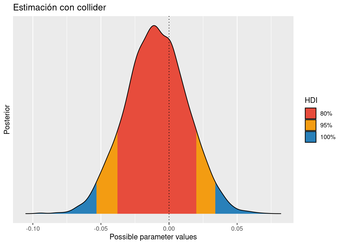
Así, que siendo “pluralista”, estimar el dag completo nos puede ayudar en situaciones dónde el backdoor criterio nos diga que no se puede estimar el efecto causal.