library(tidyverse)
library(DT)
df <-  read_csv(here::here("data/encuestas_agregadas.csv")) |>
    select(empresa, time, partido, everything())

datatable(df)Meta-análisis. Agregando encuestas
muestreo
2023
encuestas electorales
análisis bayesiano
Introducción
Ya en 2022 os mostraba uno de los ingredientes principales de la cocina electoral, al menos de la tradicional, no de la postmoderna Alaminos-Tezanos.
Hoy os quiero contar como haría yo la agregación de encuestas, cuando no se tienen los datos brutos. En primer lugar aviso de lo que sigue a continuación sólo lo he hecho por diversión y faltaría mucho más trabajo para considerarlo un intento serio.
La diversión viene por este tweet de Anabel Forte que puso como contestación a un hilo dónde Kiko Llaneras explicaba su modelo de predicción agregando encuestas y haciendo simulaciones. Aquí el hilo de kiko y en la imagen la respuesta de Ana.

Total, que dado que conozco a Ana y a Virgilio y son bayesianos y yo sólo un aprendiz de la cosa, pues he intentado un metaanálisis bayesiano sencillo juntando varias encuestas.
Datos
Lo primero era intentar encontrar datos de las encuestas que se han hecho, importante que tengan tanto la estimación como el tamaño muestral. Si, ya sé que cada empresa tiene su cocina y sus cosas, que unas son telefónicas, que otras son tracking o paneles y tal, pero ya he dicho que lo estoy haciendo por diversión..
Bueno, pues aquí he encontrado la info que buscaba. El tema es que la tabla está en una tabla de datawrapper enlace_table y no he sido capaz de escrapear de forma programática, que se le va a hacer, no vale uno pa to.
Como eran muchas encuestas pues he ido seleccionando algunas del mes de julio y al final me he quedado con unas 23. Para cada encuesta he puesto su tamaño muestral, la diferencia entre la fecha de las elecciones y la fecha de la realización de la encuesta, variable time , también he convertido a votos la estimación que dan para pp, psoe, sumar, vox y resto, simplemente multiplicando la estimación que dan por su tamaño muestral.
Mejor vemos la tabla
Pintamos
colores <-  c(
    "pp" = "#005999",
    "psoe" = "#FF0126",
    "sumar" = "#A00B85",
    "vox" = "#51962A",
    "resto" = "grey"
    )

df |>
    ggplot(aes(x = time, y = estim,color = partido )) +
    geom_point() +
    scale_color_manual(values = colores) +
    geom_smooth(se = FALSE)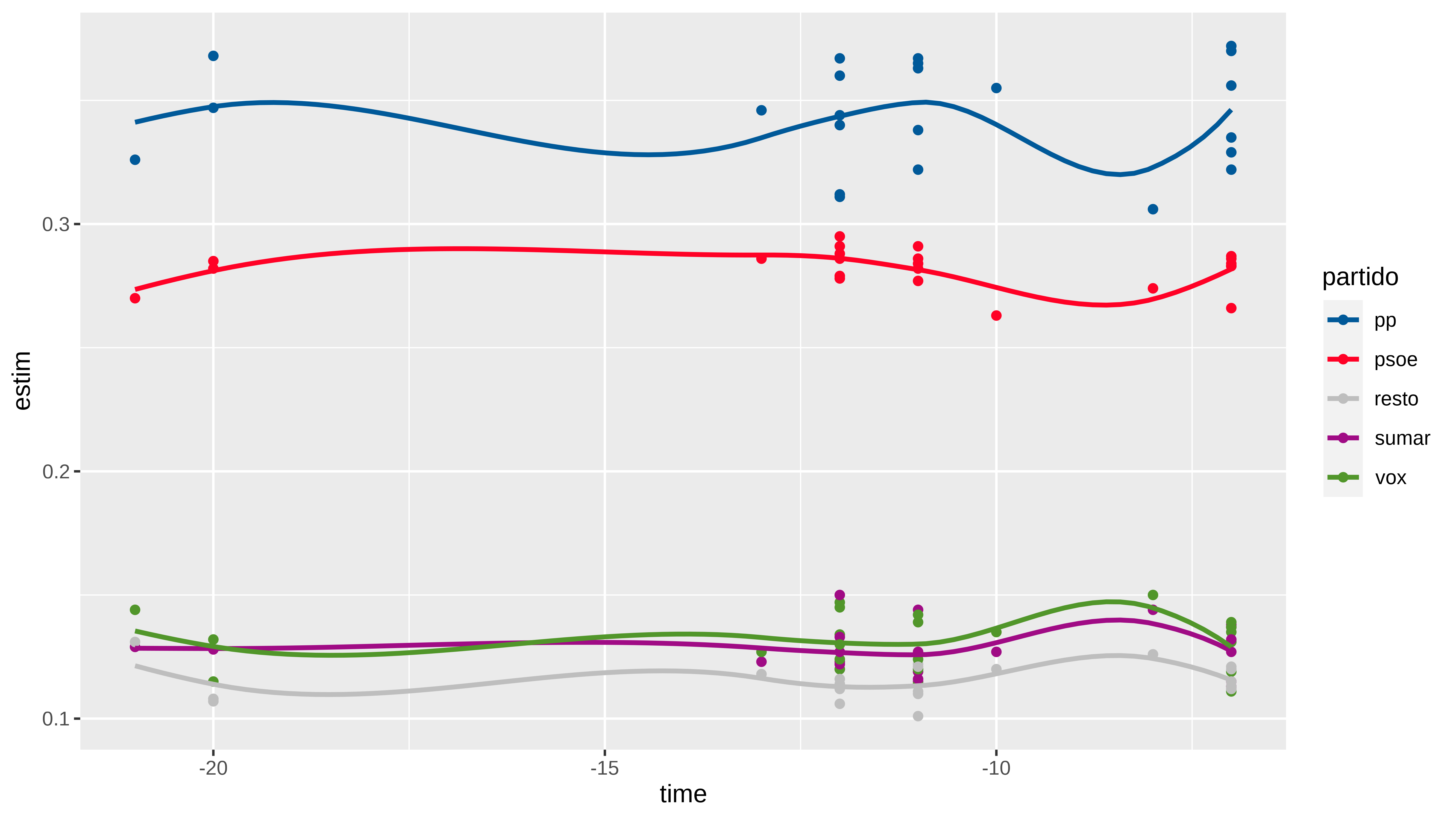
La selección de encuestas la he hecho sin mucho orden, son todas del mes de julio, algunas empresas repiten como sigma2 , gad3, simple_logica o sociométrica, otras veces he puesto como nombre el medio (okdiario o prisa).
Bueno, pues vamos a ver como hago el metaanálisis.
Preparación datos
Voy a poner los datos en un formato que me conviene más para lo que quiero hacer.
- n es tamaño de muestra
- time : es días hasta elecciones, -7 quiere decir qeu la encuesta se publicó (o se hizo, no lo sé) 7 días antes del 23 de julio
- Columnas resultantes de multiplicar la estimación en la encuesta para cada partido por el tamaño muestral
Como vemos voy a considerar 23 encuestas.
df_wider <- df |>
    select(-estim) |>
    pivot_wider( id_cols = c(empresa, n, time),
                 names_from = partido,
                 values_from = votos) |>
    arrange(empresa)

DT::datatable(df_wider)
Pues con esto ya puedo hacer mi intento de meta-análisis, que es probable que esté mal, que no soy un experto en estas cosas.
Meta-análisis
Pues lo voy a hacer de forma bayesiana. Los datos los tenemos a nivel de encuesta, por lo que puedo considerar que los votos estimados a cada partido en cada encuesta siguen una distribución multinomial , dónde n (tamaño muestral) es el número de intentos y tengo el vector de votos a cada partido que se obtendría. La suma de pp+psoe+sumar+vox+resto es igual a n para cada fila de los datos.
También puedo considerar que las estimaciones de varias encuestas realizadas por la misma empresa no son independientes, no es descabellado ¿verdad?. Y también podría considerar que las estimaciones varían conforme se acerca la fecha de las elecciones y que esta variación podría ser diferente para cada empresa encuestadora. Pues con estos ingredientes ya puedo hacer el “meta-análisis”
Utilizo la librería brms que me va a permitir hacerlo con una interfaz sencilla. Y en algún momento del futuro miraré como hacerlo con numpyro que me está picando con eso Carlos
library(cmdstanr)
library(brms)
library(tidybayes)

options(brms.backend="cmdstanr")
Creamos una columna que una las columnas de los votos a partidos para que sea nuestro vector de respuesta multinomial
df_wider$cell_counts <- with(df_wider, cbind(pp, psoe,sumar, vox, resto))

DT::datatable(head(df_wider))
Y pasamos a ajustar el modelo, dónde vamos a considerar como efecto aleatorio la empresa y como efecto fijo el tiempo, aunque diferente para cada empresa.
En la fórmula de brms añadimos informacióna la variable respuesta, en este caso añadimos la info del tamaño muestral. Mirando cosas sobre meta-análisis con brms se puede añadir cosas como desviación estándar de la estimación del efecto y cosas así.
formula <- brmsformula(
    cell_counts | trials(n) ~  (time |empresa))

# vemos las priors por defecto qeu h
(priors <- get_prior(formula, df_wider, family = multinomial()))
#>                 prior     class      coef   group resp    dpar nlpar lb ub
#>                lkj(1)       cor
#>                lkj(1)       cor           empresa
#>                (flat) Intercept
#>  student_t(3, 0, 2.5) Intercept                         mupsoe
#>  student_t(3, 0, 2.5)        sd                         mupsoe        0
#>  student_t(3, 0, 2.5)        sd           empresa       mupsoe        0
#>  student_t(3, 0, 2.5)        sd Intercept empresa       mupsoe        0
#>  student_t(3, 0, 2.5)        sd      time empresa       mupsoe        0
#>  student_t(3, 0, 2.5) Intercept                        muresto
#>  student_t(3, 0, 2.5)        sd                        muresto        0
#>  student_t(3, 0, 2.5)        sd           empresa      muresto        0
#>  student_t(3, 0, 2.5)        sd Intercept empresa      muresto        0
#>  student_t(3, 0, 2.5)        sd      time empresa      muresto        0
#>  student_t(3, 0, 2.5) Intercept                        musumar
#>  student_t(3, 0, 2.5)        sd                        musumar        0
#>  student_t(3, 0, 2.5)        sd           empresa      musumar        0
#>  student_t(3, 0, 2.5)        sd Intercept empresa      musumar        0
#>  student_t(3, 0, 2.5)        sd      time empresa      musumar        0
#>  student_t(3, 0, 2.5) Intercept                          muvox
#>  student_t(3, 0, 2.5)        sd                          muvox        0
#>  student_t(3, 0, 2.5)        sd           empresa        muvox        0
#>  student_t(3, 0, 2.5)        sd Intercept empresa        muvox        0
#>  student_t(3, 0, 2.5)        sd      time empresa        muvox        0
#>        source
#>       default
#>  (vectorized)
#>       default
#>       default
#>       default
#>  (vectorized)
#>  (vectorized)
#>  (vectorized)
#>       default
#>       default
#>  (vectorized)
#>  (vectorized)
#>  (vectorized)
#>       default
#>       default
#>  (vectorized)
#>  (vectorized)
#>  (vectorized)
#>       default
#>       default
#>  (vectorized)
#>  (vectorized)
#>  (vectorized)
Ajustamos el modelo
model_multinomial <-
    brm(
        formula,
        df_wider,
        multinomial(),
        prior = priors,
        iter = 4000,
        warmup = 1000,
        cores = 4,
        chains = 4,
        seed = 47,
        backend = "cmdstanr",
        control = list(adapt_delta = 0.95),
        refresh = 0
    )
#> Running MCMC with 4 parallel chains...
#>
#> Chain 1 finished in 8.5 seconds.
#> Chain 3 finished in 8.6 seconds.
#> Chain 4 finished in 8.7 seconds.
#> Chain 2 finished in 9.7 seconds.
#>
#> All 4 chains finished successfully.
#> Mean chain execution time: 8.9 seconds.
#> Total execution time: 9.8 seconds.

summary(model_multinomial)
#>  Family: multinomial
#>   Links: mupsoe = logit; musumar = logit; muvox = logit; muresto = logit
#> Formula: cell_counts | trials(n) ~ (time | empresa)
#>    Data: df_wider (Number of observations: 23)
#>   Draws: 4 chains, each with iter = 4000; warmup = 1000; thin = 1;
#>          total post-warmup draws = 12000
#>
#> Group-Level Effects:
#> ~empresa (Number of levels: 10)
#>                                     Estimate Est.Error l-95% CI u-95% CI Rhat
#> sd(mupsoe_Intercept)                    0.05      0.03     0.00     0.13 1.00
#> sd(mupsoe_time)                         0.00      0.00     0.00     0.01 1.00
#> sd(musumar_Intercept)                   0.14      0.06     0.05     0.28 1.00
#> sd(musumar_time)                        0.00      0.00     0.00     0.02 1.00
#> sd(muvox_Intercept)                     0.11      0.06     0.01     0.25 1.00
#> sd(muvox_time)                          0.01      0.01     0.00     0.02 1.00
#> sd(muresto_Intercept)                   0.05      0.04     0.00     0.16 1.00
#> sd(muresto_time)                        0.01      0.00     0.00     0.01 1.00
#> cor(mupsoe_Intercept,mupsoe_time)       0.06      0.58    -0.94     0.95 1.00
#> cor(musumar_Intercept,musumar_time)     0.28      0.56    -0.88     0.98 1.00
#> cor(muvox_Intercept,muvox_time)        -0.03      0.56    -0.95     0.93 1.00
#> cor(muresto_Intercept,muresto_time)     0.21      0.58    -0.91     0.98 1.00
#>                                     Bulk_ESS Tail_ESS
#> sd(mupsoe_Intercept)                    3451     3599
#> sd(mupsoe_time)                         2876     5041
#> sd(musumar_Intercept)                   3697     3162
#> sd(musumar_time)                        3236     4666
#> sd(muvox_Intercept)                     2951     2225
#> sd(muvox_time)                          1842     4433
#> sd(muresto_Intercept)                   5233     4971
#> sd(muresto_time)                        3078     3653
#> cor(mupsoe_Intercept,mupsoe_time)       5869     6716
#> cor(musumar_Intercept,musumar_time)     7015     7025
#> cor(muvox_Intercept,muvox_time)         6490     6740
#> cor(muresto_Intercept,muresto_time)     4284     6808
#>
#> Population-Level Effects:
#>                   Estimate Est.Error l-95% CI u-95% CI Rhat Bulk_ESS Tail_ESS
#> mupsoe_Intercept     -0.20      0.03    -0.25    -0.15 1.00     6469     6941
#> musumar_Intercept    -0.99      0.05    -1.09    -0.90 1.00     4232     5876
#> muvox_Intercept      -0.97      0.05    -1.06    -0.87 1.00     3835     6313
#> muresto_Intercept    -1.10      0.03    -1.15    -1.04 1.00     7182     7017
#>
#> Draws were sampled using sample(hmc). For each parameter, Bulk_ESS
#> and Tail_ESS are effective sample size measures, and Rhat is the potential
#> scale reduction factor on split chains (at convergence, Rhat = 1).
Y ya tendríamos el modelo.
¿Predicción / estimación?
Vuelvo a decir que esto es sólo por diversión, para hacer algo serio tendría que haber usado mayor número de encuestas y realizadas en diferentes momentos del tiempo, tener las estimaciones que daban en cada provincia y realizar la estimación de escaños. Todo eso y más ya lo hace, y muy bien, Kiko Llaneras para El País
¿Cómo podríamos estimar lo que va a pasar el día de las elecciones con este modelo?
Pues podríamos considerar que las elecciones fueran una encuesta realizada por una empresa que no tengo en los datos (un nuevo nivel de la variable empresa) , en este caso el gobierno, y ponemos la variable time = 0
# pongo n = 1 para que me devuelva las probabilidades , si ponenemos n = 15000000 nos devolvería una # estimación de cuántos votos van a cada partido

newdata <- tibble(
    empresa = "votaciones_dia_23",
    time = 0,
    n= 1)

newdata
#> # A tibble: 1 × 3
#>   empresa            time     n
#>   <chr>             <dbl> <dbl>
#> 1 votaciones_dia_23     0     1
Ahora utilizando una función de la librería tidybayes tenemos una forma fácil de añadir las posterior predict
estimaciones <-  newdata %>%
    add_epred_draws(model_multinomial, allow_new_levels = TRUE) %>%
    mutate(partido = as_factor(.category)) |>
    select(-.category)

dim(estimaciones )
#> [1] 60000    10

DT::datatable(head(estimaciones, 100))
Y tenemos 12000 estimaciones de la posteriori para cada partido. Esto se podría decir que es equivalente a las 15000 simulaciones que hace Kiko con su modelo. Bueno, salvo que él en cada simulación calcula más cosas, como los escaños obtenidos etc..
Podemos hacer un summary de las posteriores y ver intervalo de credibilidad al 80% por ejemplo
estimaciones |>
    group_by(partido) |>
    summarise(
        media = mean(.epred),
        mediana= median(.epred),
        low = quantile(.epred, 0.05),
        high= quantile(.epred, 0.95)
    )
#> # A tibble: 5 × 5
#>   partido media mediana   low  high
#>   <fct>   <dbl>   <dbl> <dbl> <dbl>
#> 1 pp      0.344   0.344 0.324 0.364
#> 2 psoe    0.282   0.282 0.265 0.298
#> 3 sumar   0.128   0.127 0.110 0.148
#> 4 vox     0.131   0.131 0.116 0.148
#> 5 resto   0.115   0.115 0.105 0.125
O pintar las distribuciones. .
estimaciones %>%
    ggplot(aes(x=.epred, fill = partido)) +
    geom_density(alpha = 0.5 ) +
    scale_x_continuous(labels = scales::percent) +
    scale_fill_manual(values = colores) +
    labs(title="Agregando encuestas por diversión. Resultado",
        x = "Porcentaje estimado",
        y = "Density")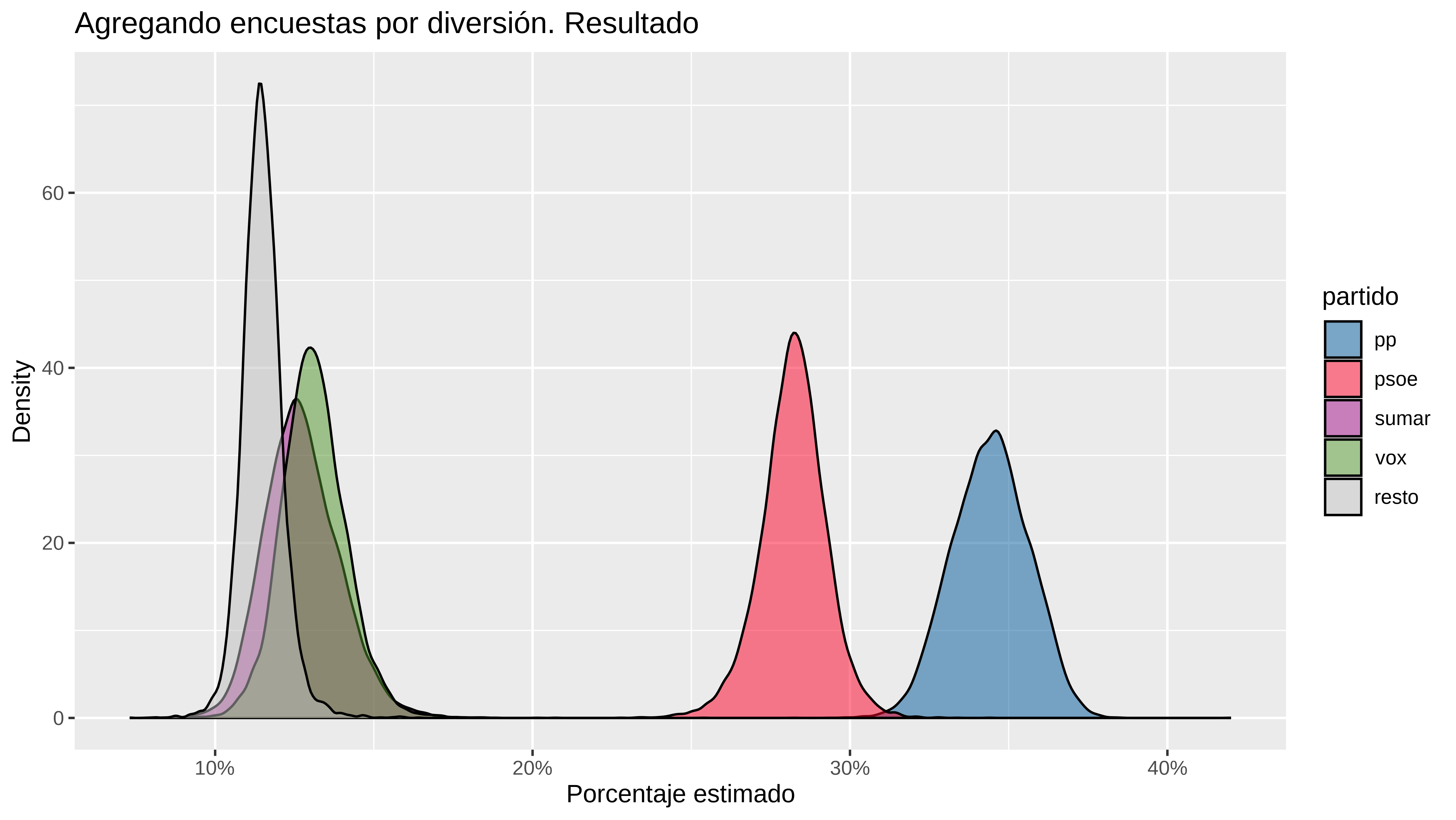
¿Qué más cosas podemos hacer? Ya que tengo las posterioris puedo usarlas y calcular las posterioris del bloque PP+ Vox o de cualquier otra cosa.
Supongamos que hubiera 15 millones de votos válidos.
votantes <- 15e6
posterioris <- estimaciones  |>
    ungroup() |>
    mutate(votos = votantes * .epred) |>
    select(partido, votos) |>
    pivot_wider(names_from = partido, values_from = votos)

# tenemos columnas que son listas.  hay que hacer un unnest
posterioris
#> # A tibble: 1 × 5
#>   pp             psoe           sumar          vox            resto
#>   <list>         <list>         <list>         <list>         <list>
#> 1 <dbl [12,000]> <dbl [12,000]> <dbl [12,000]> <dbl [12,000]> <dbl [12,000]>
posterioris <- posterioris |>
unnest(c(pp, psoe, sumar, vox, resto))
head(posterioris)
#> # A tibble: 6 × 5
#> pp psoe sumar vox resto
#> <dbl> <dbl> <dbl> <dbl> <dbl>
#> 1 5023147. 4400631. 1873502. 2108276. 1594443.
#> 2 5402129. 4297818. 1791318. 1783497. 1725237.
#> 3 5066890. 4415547. 1741994. 1990458. 1785111.
#> 4 5372578. 4119759. 1768716. 1833665. 1905282.
#> 5 5022623. 4342021. 2004152. 1986356. 1644848.
#> 6 5287214. 4283855. 1876413. 1714759. 1837759.Sumo votos de los bloques para cada una de las 12000 filas. Además. añado al bloque de la izquierda el 50% de los votos que están en resto.
posterioris <- posterioris |>
    mutate(
        derecha = pp + vox,
        izquierda = psoe + sumar + 0.5*resto) |>
    mutate(derecha_posterior = derecha / votantes,
           izquierda_posterior = izquierda/votantes)

posterioris |>
    head(20)
#> # A tibble: 20 × 9
#>          pp     psoe    sumar     vox  resto derecha izquierda derecha_posterior
#>       <dbl>    <dbl>    <dbl>   <dbl>  <dbl>   <dbl>     <dbl>             <dbl>
#>  1 5023147. 4400631. 1873502.  2.11e6 1.59e6  7.13e6  7071355.             0.475
#>  2 5402129. 4297818. 1791318.  1.78e6 1.73e6  7.19e6  6951755.             0.479
#>  3 5066890. 4415547. 1741994.  1.99e6 1.79e6  7.06e6  7050097.             0.470
#>  4 5372578. 4119759. 1768716.  1.83e6 1.91e6  7.21e6  6841116.             0.480
#>  5 5022623. 4342021. 2004152.  1.99e6 1.64e6  7.01e6  7168597.             0.467
#>  6 5287214. 4283855. 1876413.  1.71e6 1.84e6  7.00e6  7079147.             0.467
#>  7 5017396. 4110837. 2085376.  2.23e6 1.56e6  7.25e6  6974129.             0.483
#>  8 4793459. 4479950. 2223135.  2.01e6 1.49e6  6.80e6  7449523.             0.454
#>  9 5345670. 4142111. 1795447.  2.03e6 1.69e6  7.38e6  6781142.             0.492
#> 10 5127698. 4210917. 1935521.  1.91e6 1.82e6  7.04e6  7055529.             0.469
#> 11 5486238. 4199075. 1588582.  1.86e6 1.87e6  7.35e6  6720877.             0.490
#> 12 5149876. 4219835. 2100181.  1.78e6 1.75e6  6.93e6  7193195.             0.462
#> 13 4759372. 4465230. 2329286.  1.84e6 1.60e6  6.60e6  7596283.             0.440
#> 14 5236625. 4338129. 1747429.  1.95e6 1.73e6  7.18e6  6950958.             0.479
#> 15 5206440. 4387667. 1749035.  1.99e6 1.67e6  7.19e6  6971347.             0.480
#> 16 4854678. 4329145. 2184347.  1.77e6 1.86e6  6.62e6  7444375.             0.442
#> 17 5250217. 4518969. 1701659.  1.75e6 1.78e6  7.00e6  7110288.             0.467
#> 18 5179197. 4451222. 1814213.  1.79e6 1.76e6  6.97e6  7147712.             0.465
#> 19 4807230. 4425101. 1768384.  2.44e6 1.56e6  7.25e6  6974064.             0.483
#> 20 5001895. 3986637. 2109063.  2.05e6 1.85e6  7.05e6  7022137.             0.470
#> # ℹ 1 more variable: izquierda_posterior <dbl>
Ahora nos podemos hacer preguntas como , ¿en cuántas de estas posterioris gana el bloque de la derecha así construido al de la izquierda? o ¿en cuántas la diferencia que le saca el bloque de la derecha es mayor a un punto porcentual?
posterioris |>
    mutate(gana_derecha = derecha_posterior>izquierda_posterior,
           gana_derecha_mas1_pct = (derecha_posterior - izquierda_posterior) >= 0.01) |>
    summarise(
        mean(gana_derecha),
        mean(gana_derecha_mas1_pct)
        )
#> # A tibble: 1 × 2
#>   `mean(gana_derecha)` `mean(gana_derecha_mas1_pct)`
#>                  <dbl>                         <dbl>
#> 1                0.673                         0.480
Actualización [2023-07-24]
Ya fueron las elecciones generales y escrutado al 100% se tiene que
Y claramente el promedio de encuestas infraestimó el voto al psoe. Para pp, sumar o o vox si que acertaron relativamente bien, aunque pp y vox se han quedado más cerda del extremo inferior del intervalo que del punto medio.
¿Si hubiera considerado más encuestas habría cambiado algo?
df_update <-  read_csv(here::here("data/encuestas_agregadas_39.csv")) |>
    select(empresa, time, partido, everything())
# Añado botones para descarga de datos
datatable(df, extensions = "Buttons",
          options = list(
              dom = 'Bfrtip',
              buttons = c('copy', 'csv', 'excel', 'pdf') )
          )
df_wider <- df_update |>
    select(-estim) |>
    pivot_wider( id_cols = c(empresa, n, time),
                 names_from = partido,
                 values_from = votos) |>
    arrange(empresa)

df_wider$cell_counts <- with(df_wider, cbind(resto,pp, psoe,sumar, vox))

DT::datatable(df_wider)
# cambio un poco la formla pq quiero efecto fijo del tiempo además del varying
# slope
formula <- brmsformula(
    cell_counts | trials(n) ~ time +  (time |empresa))

model_multinomial_update <- brm(formula, df_wider, multinomial(),
                          iter = 4000, warmup = 1000, cores = 4, chains = 4,
                          seed = 3,
                          backend = "cmdstanr",
                         control = list(adapt_delta = 0.95)
)
#> Running MCMC with 4 parallel chains...
#>
#> Chain 1 Iteration:    1 / 4000 [  0%]  (Warmup)
#> Chain 2 Iteration:    1 / 4000 [  0%]  (Warmup)
#> Chain 3 Iteration:    1 / 4000 [  0%]  (Warmup)
#> Chain 4 Iteration:    1 / 4000 [  0%]  (Warmup)
#> Chain 3 Iteration:  100 / 4000 [  2%]  (Warmup)
#> Chain 1 Iteration:  100 / 4000 [  2%]  (Warmup)
#> Chain 2 Iteration:  100 / 4000 [  2%]  (Warmup)
#> Chain 4 Iteration:  100 / 4000 [  2%]  (Warmup)
#> Chain 3 Iteration:  200 / 4000 [  5%]  (Warmup)
#> Chain 1 Iteration:  200 / 4000 [  5%]  (Warmup)
#> Chain 2 Iteration:  200 / 4000 [  5%]  (Warmup)
#> Chain 3 Iteration:  300 / 4000 [  7%]  (Warmup)
#> Chain 4 Iteration:  200 / 4000 [  5%]  (Warmup)
#> Chain 3 Iteration:  400 / 4000 [ 10%]  (Warmup)
#> Chain 2 Iteration:  300 / 4000 [  7%]  (Warmup)
#> Chain 1 Iteration:  300 / 4000 [  7%]  (Warmup)
#> Chain 2 Iteration:  400 / 4000 [ 10%]  (Warmup)
#> Chain 3 Iteration:  500 / 4000 [ 12%]  (Warmup)
#> Chain 4 Iteration:  300 / 4000 [  7%]  (Warmup)
#> Chain 1 Iteration:  400 / 4000 [ 10%]  (Warmup)
#> Chain 3 Iteration:  600 / 4000 [ 15%]  (Warmup)
#> Chain 2 Iteration:  500 / 4000 [ 12%]  (Warmup)
#> Chain 4 Iteration:  400 / 4000 [ 10%]  (Warmup)
#> Chain 1 Iteration:  500 / 4000 [ 12%]  (Warmup)
#> Chain 3 Iteration:  700 / 4000 [ 17%]  (Warmup)
#> Chain 2 Iteration:  600 / 4000 [ 15%]  (Warmup)
#> Chain 1 Iteration:  600 / 4000 [ 15%]  (Warmup)
#> Chain 3 Iteration:  800 / 4000 [ 20%]  (Warmup)
#> Chain 4 Iteration:  500 / 4000 [ 12%]  (Warmup)
#> Chain 2 Iteration:  700 / 4000 [ 17%]  (Warmup)
#> Chain 1 Iteration:  700 / 4000 [ 17%]  (Warmup)
#> Chain 3 Iteration:  900 / 4000 [ 22%]  (Warmup)
#> Chain 4 Iteration:  600 / 4000 [ 15%]  (Warmup)
#> Chain 2 Iteration:  800 / 4000 [ 20%]  (Warmup)
#> Chain 1 Iteration:  800 / 4000 [ 20%]  (Warmup)
#> Chain 3 Iteration: 1000 / 4000 [ 25%]  (Warmup)
#> Chain 3 Iteration: 1001 / 4000 [ 25%]  (Sampling)
#> Chain 4 Iteration:  700 / 4000 [ 17%]  (Warmup)
#> Chain 2 Iteration:  900 / 4000 [ 22%]  (Warmup)
#> Chain 1 Iteration:  900 / 4000 [ 22%]  (Warmup)
#> Chain 3 Iteration: 1100 / 4000 [ 27%]  (Sampling)
#> Chain 4 Iteration:  800 / 4000 [ 20%]  (Warmup)
#> Chain 1 Iteration: 1000 / 4000 [ 25%]  (Warmup)
#> Chain 1 Iteration: 1001 / 4000 [ 25%]  (Sampling)
#> Chain 2 Iteration: 1000 / 4000 [ 25%]  (Warmup)
#> Chain 2 Iteration: 1001 / 4000 [ 25%]  (Sampling)
#> Chain 3 Iteration: 1200 / 4000 [ 30%]  (Sampling)
#> Chain 4 Iteration:  900 / 4000 [ 22%]  (Warmup)
#> Chain 1 Iteration: 1100 / 4000 [ 27%]  (Sampling)
#> Chain 2 Iteration: 1100 / 4000 [ 27%]  (Sampling)
#> Chain 3 Iteration: 1300 / 4000 [ 32%]  (Sampling)
#> Chain 4 Iteration: 1000 / 4000 [ 25%]  (Warmup)
#> Chain 4 Iteration: 1001 / 4000 [ 25%]  (Sampling)
#> Chain 1 Iteration: 1200 / 4000 [ 30%]  (Sampling)
#> Chain 2 Iteration: 1200 / 4000 [ 30%]  (Sampling)
#> Chain 3 Iteration: 1400 / 4000 [ 35%]  (Sampling)
#> Chain 4 Iteration: 1100 / 4000 [ 27%]  (Sampling)
#> Chain 2 Iteration: 1300 / 4000 [ 32%]  (Sampling)
#> Chain 1 Iteration: 1300 / 4000 [ 32%]  (Sampling)
#> Chain 3 Iteration: 1500 / 4000 [ 37%]  (Sampling)
#> Chain 4 Iteration: 1200 / 4000 [ 30%]  (Sampling)
#> Chain 2 Iteration: 1400 / 4000 [ 35%]  (Sampling)
#> Chain 1 Iteration: 1400 / 4000 [ 35%]  (Sampling)
#> Chain 3 Iteration: 1600 / 4000 [ 40%]  (Sampling)
#> Chain 4 Iteration: 1300 / 4000 [ 32%]  (Sampling)
#> Chain 1 Iteration: 1500 / 4000 [ 37%]  (Sampling)
#> Chain 2 Iteration: 1500 / 4000 [ 37%]  (Sampling)
#> Chain 3 Iteration: 1700 / 4000 [ 42%]  (Sampling)
#> Chain 4 Iteration: 1400 / 4000 [ 35%]  (Sampling)
#> Chain 1 Iteration: 1600 / 4000 [ 40%]  (Sampling)
#> Chain 2 Iteration: 1600 / 4000 [ 40%]  (Sampling)
#> Chain 3 Iteration: 1800 / 4000 [ 45%]  (Sampling)
#> Chain 4 Iteration: 1500 / 4000 [ 37%]  (Sampling)
#> Chain 1 Iteration: 1700 / 4000 [ 42%]  (Sampling)
#> Chain 2 Iteration: 1700 / 4000 [ 42%]  (Sampling)
#> Chain 3 Iteration: 1900 / 4000 [ 47%]  (Sampling)
#> Chain 4 Iteration: 1600 / 4000 [ 40%]  (Sampling)
#> Chain 2 Iteration: 1800 / 4000 [ 45%]  (Sampling)
#> Chain 1 Iteration: 1800 / 4000 [ 45%]  (Sampling)
#> Chain 3 Iteration: 2000 / 4000 [ 50%]  (Sampling)
#> Chain 4 Iteration: 1700 / 4000 [ 42%]  (Sampling)
#> Chain 2 Iteration: 1900 / 4000 [ 47%]  (Sampling)
#> Chain 1 Iteration: 1900 / 4000 [ 47%]  (Sampling)
#> Chain 3 Iteration: 2100 / 4000 [ 52%]  (Sampling)
#> Chain 4 Iteration: 1800 / 4000 [ 45%]  (Sampling)
#> Chain 2 Iteration: 2000 / 4000 [ 50%]  (Sampling)
#> Chain 1 Iteration: 2000 / 4000 [ 50%]  (Sampling)
#> Chain 3 Iteration: 2200 / 4000 [ 55%]  (Sampling)
#> Chain 4 Iteration: 1900 / 4000 [ 47%]  (Sampling)
#> Chain 1 Iteration: 2100 / 4000 [ 52%]  (Sampling)
#> Chain 2 Iteration: 2100 / 4000 [ 52%]  (Sampling)
#> Chain 3 Iteration: 2300 / 4000 [ 57%]  (Sampling)
#> Chain 4 Iteration: 2000 / 4000 [ 50%]  (Sampling)
#> Chain 1 Iteration: 2200 / 4000 [ 55%]  (Sampling)
#> Chain 2 Iteration: 2200 / 4000 [ 55%]  (Sampling)
#> Chain 3 Iteration: 2400 / 4000 [ 60%]  (Sampling)
#> Chain 4 Iteration: 2100 / 4000 [ 52%]  (Sampling)
#> Chain 1 Iteration: 2300 / 4000 [ 57%]  (Sampling)
#> Chain 2 Iteration: 2300 / 4000 [ 57%]  (Sampling)
#> Chain 3 Iteration: 2500 / 4000 [ 62%]  (Sampling)
#> Chain 4 Iteration: 2200 / 4000 [ 55%]  (Sampling)
#> Chain 2 Iteration: 2400 / 4000 [ 60%]  (Sampling)
#> Chain 1 Iteration: 2400 / 4000 [ 60%]  (Sampling)
#> Chain 3 Iteration: 2600 / 4000 [ 65%]  (Sampling)
#> Chain 4 Iteration: 2300 / 4000 [ 57%]  (Sampling)
#> Chain 2 Iteration: 2500 / 4000 [ 62%]  (Sampling)
#> Chain 1 Iteration: 2500 / 4000 [ 62%]  (Sampling)
#> Chain 3 Iteration: 2700 / 4000 [ 67%]  (Sampling)
#> Chain 4 Iteration: 2400 / 4000 [ 60%]  (Sampling)
#> Chain 2 Iteration: 2600 / 4000 [ 65%]  (Sampling)
#> Chain 1 Iteration: 2600 / 4000 [ 65%]  (Sampling)
#> Chain 3 Iteration: 2800 / 4000 [ 70%]  (Sampling)
#> Chain 4 Iteration: 2500 / 4000 [ 62%]  (Sampling)
#> Chain 1 Iteration: 2700 / 4000 [ 67%]  (Sampling)
#> Chain 2 Iteration: 2700 / 4000 [ 67%]  (Sampling)
#> Chain 3 Iteration: 2900 / 4000 [ 72%]  (Sampling)
#> Chain 4 Iteration: 2600 / 4000 [ 65%]  (Sampling)
#> Chain 1 Iteration: 2800 / 4000 [ 70%]  (Sampling)
#> Chain 2 Iteration: 2800 / 4000 [ 70%]  (Sampling)
#> Chain 3 Iteration: 3000 / 4000 [ 75%]  (Sampling)
#> Chain 4 Iteration: 2700 / 4000 [ 67%]  (Sampling)
#> Chain 2 Iteration: 2900 / 4000 [ 72%]  (Sampling)
#> Chain 1 Iteration: 2900 / 4000 [ 72%]  (Sampling)
#> Chain 3 Iteration: 3100 / 4000 [ 77%]  (Sampling)
#> Chain 4 Iteration: 2800 / 4000 [ 70%]  (Sampling)
#> Chain 2 Iteration: 3000 / 4000 [ 75%]  (Sampling)
#> Chain 1 Iteration: 3000 / 4000 [ 75%]  (Sampling)
#> Chain 3 Iteration: 3200 / 4000 [ 80%]  (Sampling)
#> Chain 4 Iteration: 2900 / 4000 [ 72%]  (Sampling)
#> Chain 1 Iteration: 3100 / 4000 [ 77%]  (Sampling)
#> Chain 2 Iteration: 3100 / 4000 [ 77%]  (Sampling)
#> Chain 3 Iteration: 3300 / 4000 [ 82%]  (Sampling)
#> Chain 4 Iteration: 3000 / 4000 [ 75%]  (Sampling)
#> Chain 1 Iteration: 3200 / 4000 [ 80%]  (Sampling)
#> Chain 2 Iteration: 3200 / 4000 [ 80%]  (Sampling)
#> Chain 3 Iteration: 3400 / 4000 [ 85%]  (Sampling)
#> Chain 4 Iteration: 3100 / 4000 [ 77%]  (Sampling)
#> Chain 2 Iteration: 3300 / 4000 [ 82%]  (Sampling)
#> Chain 1 Iteration: 3300 / 4000 [ 82%]  (Sampling)
#> Chain 3 Iteration: 3500 / 4000 [ 87%]  (Sampling)
#> Chain 4 Iteration: 3200 / 4000 [ 80%]  (Sampling)
#> Chain 1 Iteration: 3400 / 4000 [ 85%]  (Sampling)
#> Chain 2 Iteration: 3400 / 4000 [ 85%]  (Sampling)
#> Chain 3 Iteration: 3600 / 4000 [ 90%]  (Sampling)
#> Chain 4 Iteration: 3300 / 4000 [ 82%]  (Sampling)
#> Chain 1 Iteration: 3500 / 4000 [ 87%]  (Sampling)
#> Chain 2 Iteration: 3500 / 4000 [ 87%]  (Sampling)
#> Chain 3 Iteration: 3700 / 4000 [ 92%]  (Sampling)
#> Chain 4 Iteration: 3400 / 4000 [ 85%]  (Sampling)
#> Chain 1 Iteration: 3600 / 4000 [ 90%]  (Sampling)
#> Chain 2 Iteration: 3600 / 4000 [ 90%]  (Sampling)
#> Chain 3 Iteration: 3800 / 4000 [ 95%]  (Sampling)
#> Chain 4 Iteration: 3500 / 4000 [ 87%]  (Sampling)
#> Chain 1 Iteration: 3700 / 4000 [ 92%]  (Sampling)
#> Chain 2 Iteration: 3700 / 4000 [ 92%]  (Sampling)
#> Chain 3 Iteration: 3900 / 4000 [ 97%]  (Sampling)
#> Chain 4 Iteration: 3600 / 4000 [ 90%]  (Sampling)
#> Chain 1 Iteration: 3800 / 4000 [ 95%]  (Sampling)
#> Chain 2 Iteration: 3800 / 4000 [ 95%]  (Sampling)
#> Chain 3 Iteration: 4000 / 4000 [100%]  (Sampling)
#> Chain 3 finished in 24.5 seconds.
#> Chain 4 Iteration: 3700 / 4000 [ 92%]  (Sampling)
#> Chain 2 Iteration: 3900 / 4000 [ 97%]  (Sampling)
#> Chain 1 Iteration: 3900 / 4000 [ 97%]  (Sampling)
#> Chain 4 Iteration: 3800 / 4000 [ 95%]  (Sampling)
#> Chain 1 Iteration: 4000 / 4000 [100%]  (Sampling)
#> Chain 2 Iteration: 4000 / 4000 [100%]  (Sampling)
#> Chain 1 finished in 25.4 seconds.
#> Chain 2 finished in 25.4 seconds.
#> Chain 4 Iteration: 3900 / 4000 [ 97%]  (Sampling)
#> Chain 4 Iteration: 4000 / 4000 [100%]  (Sampling)
#> Chain 4 finished in 26.1 seconds.
#>
#> All 4 chains finished successfully.
#> Mean chain execution time: 25.3 seconds.
#> Total execution time: 26.2 seconds.
estimaciones_update <- newdata %>%
add_epred_draws(model_multinomial_update, allow_new_levels = TRUE) %>%
mutate(partido = as_factor(.category)) |>
select(-.category)Pues parece que no cambia mucho. Si acaso añade más incertidumbre y ahora el resultado del psoe está dentro del intervalo de credibilidad del 90%
estimaciones_update |>
    group_by(partido) |>
    summarise(
        media = mean(.epred),
        mediana= median(.epred),
        low = quantile(.epred, 0.05),
        high= quantile(.epred, 0.95)
    )
#> # A tibble: 5 × 5
#>   partido media mediana    low  high
#>   <fct>   <dbl>   <dbl>  <dbl> <dbl>
#> 1 resto   0.115   0.115 0.108  0.126
#> 2 pp      0.343   0.343 0.310  0.375
#> 3 psoe    0.292   0.290 0.275  0.322
#> 4 sumar   0.125   0.124 0.113  0.139
#> 5 vox     0.125   0.128 0.0789 0.150
estimaciones_update %>%
    ggplot(aes(x=.epred, fill = partido)) +
    geom_density(alpha = 0.5 ) +
    scale_x_continuous(labels = scales::percent) +
    scale_fill_manual(values = colores) +
    labs(title="Agregando encuestas por diversión. Resultado",
         subtitle = "Actualización con más encuestas",
        x = "Porcentaje estimado",
        y = "Density")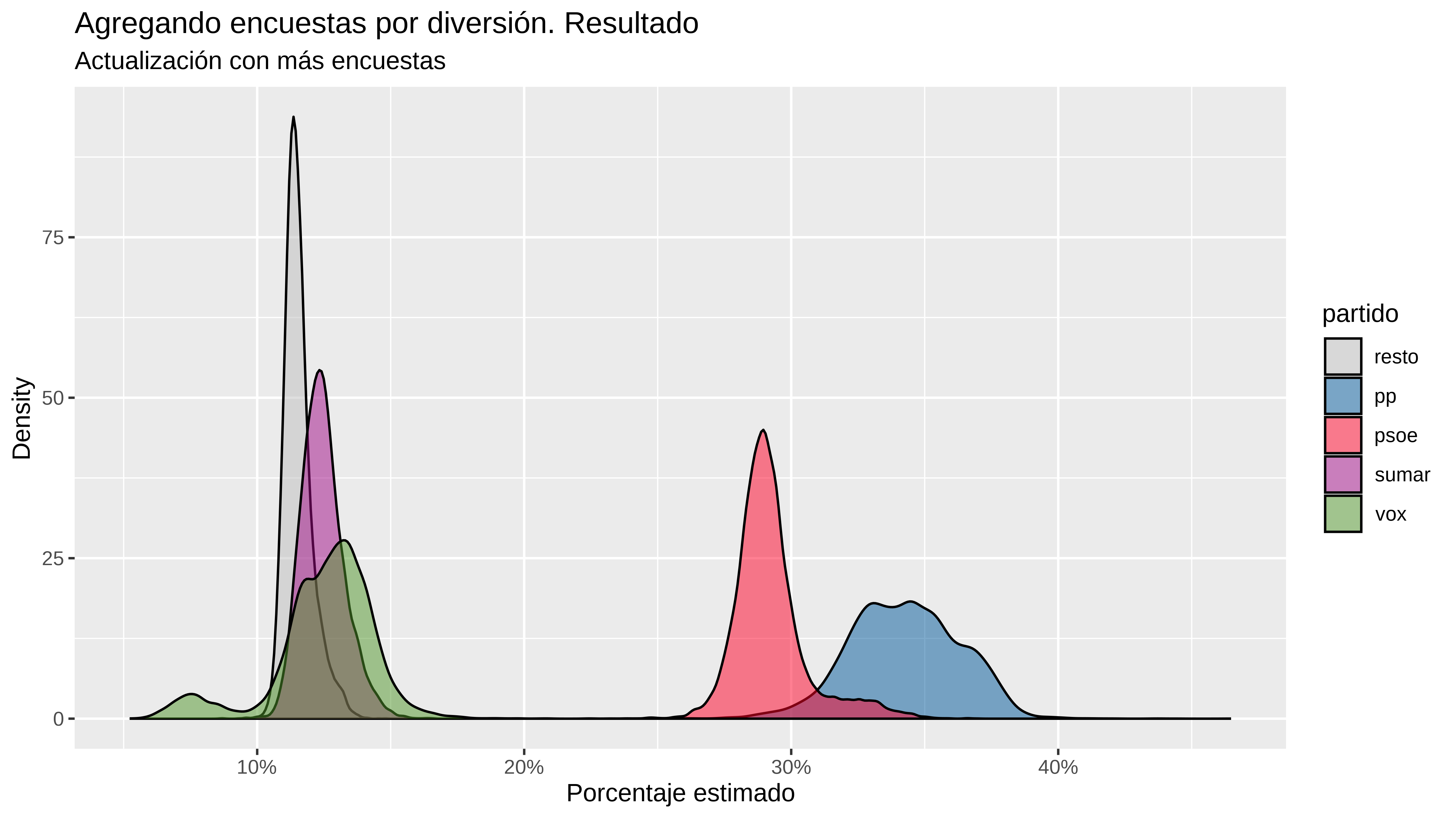
Cosas interesantes que puedo sacar del modelo. Por ejemplo los efectos aleatorios asociados a las diferentes empresas encuestadoras. Por ejemplo con mupsoe_Intercept se ve por ejemplo que la de prisa(40db) ,simple_logica (para el diario.es) sigma2 o el cis fueron las más favorables hacia el psoe.
Esto parece sugerir que los resultados de las diferentes encuestas parecen estar afectados por la mano que les da de comer.
ranef(model_multinomial_update)
#> $empresa
#> , , mupp_Intercept
#>
#>                  Estimate  Est.Error        Q2.5      Q97.5
#> celeste_tel    0.04983451 0.05847759 -0.05785386 0.17452635
#> cis           -0.11269392 0.07921043 -0.28268055 0.01887259
#> electo_mania   0.01266378 0.05495308 -0.08769483 0.12890022
#> gad3           0.12708807 0.04538762  0.04470506 0.22400860
#> gesop         -0.09336239 0.06633783 -0.23445718 0.02701568
#> invymark      -0.08845348 0.08144761 -0.26558825 0.06216075
#> nc_report      0.06977150 0.05506073 -0.03028796 0.18586357
#> ok_diario      0.04076435 0.05285644 -0.05784015 0.15009835
#> prisa         -0.02726022 0.04755849 -0.11914163 0.07052230
#> sigma2         0.03550888 0.04398473 -0.04942665 0.12580797
#> simple_logica -0.02710374 0.04962525 -0.12671515 0.06897185
#> socio_metrica -0.02427102 0.05004341 -0.12195298 0.07523895
#> target_point   0.03521051 0.09644025 -0.16213082 0.23375662
#>
#> , , mupp_time
#>
#>                    Estimate    Est.Error         Q2.5        Q97.5
#> celeste_tel    5.601833e-04 0.0010752752 -0.001462165 0.0028845335
#> cis           -1.858769e-03 0.0014818803 -0.005107945 0.0003605464
#> electo_mania   8.326875e-04 0.0013083572 -0.001403193 0.0038301443
#> gad3           6.870950e-04 0.0018649834 -0.003052465 0.0044324950
#> gesop         -6.383980e-04 0.0018839697 -0.004635597 0.0029928842
#> invymark       3.140981e-05 0.0019661982 -0.004053128 0.0040827335
#> nc_report      6.845445e-04 0.0014938625 -0.002058980 0.0040297510
#> ok_diario      5.167656e-04 0.0012166924 -0.001778642 0.0031886107
#> prisa          6.750862e-04 0.0009813955 -0.001163746 0.0027679542
#> sigma2        -3.516238e-04 0.0012475810 -0.003085294 0.0019836857
#> simple_logica -1.126181e-03 0.0010989386 -0.003559223 0.0006837115
#> socio_metrica  3.710038e-04 0.0012584726 -0.002067272 0.0031104447
#> target_point  -3.996651e-04 0.0017999138 -0.004385952 0.0030570600
#>
#> , , mupsoe_Intercept
#>
#>                   Estimate  Est.Error        Q2.5      Q97.5
#> celeste_tel   -0.002276998 0.02808656 -0.06507048 0.05559588
#> cis            0.019702197 0.04093116 -0.05067533 0.11701995
#> electo_mania   0.011364728 0.02912626 -0.03663608 0.08641640
#> gad3           0.015223792 0.02628927 -0.02780848 0.07836367
#> gesop         -0.016066261 0.03623679 -0.10444262 0.04282177
#> invymark      -0.028486511 0.04541277 -0.14301735 0.04049496
#> nc_report     -0.007220812 0.02850193 -0.07316730 0.04673424
#> ok_diario     -0.030797624 0.03886857 -0.12636292 0.02279682
#> prisa          0.009762308 0.02631351 -0.03663878 0.07402995
#> sigma2         0.011121029 0.02579794 -0.03593884 0.07250188
#> simple_logica  0.016102746 0.03142286 -0.03983507 0.08999656
#> socio_metrica -0.008354206 0.02858118 -0.07234223 0.04903350
#> target_point   0.009988969 0.03623881 -0.05608511 0.09806407
#>
#> , , mupsoe_time
#>
#>                    Estimate   Est.Error          Q2.5         Q97.5
#> celeste_tel    6.351476e-05 0.001199362 -2.456705e-03  2.396963e-03
#> cis           -3.270677e-03 0.001262601 -5.934026e-03 -9.475839e-04
#> electo_mania   1.584091e-04 0.001340476 -2.472783e-03  2.911473e-03
#> gad3          -1.278420e-03 0.001959843 -5.409934e-03  2.486353e-03
#> gesop          1.001596e-03 0.002732244 -4.253542e-03  6.961284e-03
#> invymark       3.399821e-03 0.001909472  1.128583e-05  7.474699e-03
#> nc_report      9.755046e-04 0.001750050 -2.300850e-03  4.728513e-03
#> ok_diario      2.827258e-03 0.001539038 -1.292829e-05  5.969975e-03
#> prisa         -4.973800e-04 0.001138912 -2.882389e-03  1.753342e-03
#> sigma2        -1.277384e-03 0.001435137 -4.328619e-03  1.434950e-03
#> simple_logica -2.356142e-03 0.001293664 -5.124468e-03 -7.625871e-05
#> socio_metrica  1.594284e-03 0.001489799 -1.132845e-03  4.691291e-03
#> target_point  -1.411879e-03 0.001590356 -4.812724e-03  1.507244e-03
#>
#> , , musumar_Intercept
#>
#>                    Estimate  Est.Error         Q2.5      Q97.5
#> celeste_tel   -0.0358445986 0.04957444 -0.150229100 0.04743706
#> cis            0.0132971726 0.04651727 -0.069758368 0.12317857
#> electo_mania   0.0070341761 0.04248783 -0.083039127 0.09161290
#> gad3          -0.0353641132 0.03666900 -0.115859275 0.02688924
#> gesop          0.0373218097 0.05536161 -0.054462743 0.16499042
#> invymark      -0.0089751397 0.04854726 -0.111963050 0.08780055
#> nc_report     -0.0406315429 0.04748837 -0.150190250 0.03561324
#> ok_diario     -0.0102878996 0.04171049 -0.098574120 0.07398172
#> prisa          0.0225994343 0.04031133 -0.054578180 0.10777645
#> sigma2        -0.0082246939 0.03496083 -0.080907860 0.06160265
#> simple_logica  0.0751187593 0.05402766 -0.009799251 0.18905942
#> socio_metrica -0.0002657433 0.03985462 -0.084348557 0.08278825
#> target_point  -0.0165754581 0.05666641 -0.142857825 0.09367493
#>
#> , , musumar_time
#>
#>                    Estimate    Est.Error         Q2.5        Q97.5
#> celeste_tel    3.103610e-04 0.0008602449 -0.001373319 0.0022302135
#> cis            3.347250e-04 0.0008624901 -0.001128795 0.0024411762
#> electo_mania  -6.618639e-04 0.0011008107 -0.003507239 0.0008992042
#> gad3           2.429828e-05 0.0012769107 -0.002911007 0.0026252740
#> gesop         -8.011793e-05 0.0013149711 -0.002928823 0.0027984967
#> invymark       1.338833e-04 0.0011282724 -0.002083171 0.0027425217
#> nc_report      2.097078e-04 0.0011791976 -0.002183350 0.0028841215
#> ok_diario      3.148319e-04 0.0009717670 -0.001482126 0.0026558482
#> prisa         -6.035426e-04 0.0008646081 -0.002661508 0.0007422272
#> sigma2         4.400805e-04 0.0010397252 -0.001275172 0.0030627337
#> simple_logica -7.506860e-04 0.0010609271 -0.003165005 0.0009917626
#> socio_metrica  1.864726e-05 0.0009601066 -0.002061034 0.0020858427
#> target_point   3.113929e-04 0.0011178886 -0.001753471 0.0030024427
#>
#> , , muvox_Intercept
#>
#>                   Estimate  Est.Error        Q2.5      Q97.5
#> celeste_tel   -0.027563257 0.10163227 -0.22536030  0.1727010
#> cis           -0.565764453 0.13587027 -0.84565335 -0.3140112
#> electo_mania   0.066364066 0.09618556 -0.12254760  0.2570871
#> gad3          -0.008670455 0.07859782 -0.15700788  0.1495601
#> gesop          0.147990408 0.10824879 -0.05956420  0.3635356
#> invymark       0.033535523 0.14445059 -0.24711252  0.3263141
#> nc_report     -0.070586246 0.09473895 -0.25996155  0.1156743
#> ok_diario      0.054799569 0.09046204 -0.12134520  0.2336971
#> prisa          0.119210914 0.08427223 -0.04170232  0.2898681
#> sigma2         0.054515552 0.08308845 -0.10485597  0.2270518
#> simple_logica  0.138785392 0.08591571 -0.02525560  0.3128597
#> socio_metrica  0.078037685 0.08942748 -0.09257302  0.2565346
#> target_point  -0.011986902 0.20139152 -0.41809745  0.3930733
#>
#> , , muvox_time
#>
#>                    Estimate   Est.Error         Q2.5        Q97.5
#> celeste_tel    7.203336e-04 0.001784125 -0.002744172  0.004351591
#> cis           -7.170722e-03 0.002312615 -0.011891795 -0.002824443
#> electo_mania  -1.162150e-03 0.002241739 -0.005934080  0.002965156
#> gad3           4.264346e-04 0.002470284 -0.004084816  0.005839640
#> gesop          1.762831e-03 0.002799074 -0.003799805  0.007700488
#> invymark       3.921615e-04 0.003261884 -0.006150279  0.007273604
#> nc_report     -1.506608e-03 0.002381401 -0.006585859  0.002923375
#> ok_diario      8.105272e-05 0.001922182 -0.003800808  0.003791748
#> prisa          2.484377e-03 0.001586320 -0.000466300  0.005714418
#> sigma2         2.661615e-03 0.002236228 -0.001143362  0.007573518
#> simple_logica  1.070490e-03 0.001608866 -0.002146405  0.004289484
#> socio_metrica  2.899506e-04 0.002028250 -0.003889796  0.004245027
#> target_point   7.433332e-06 0.003551183 -0.007202358  0.007231719
Coda
Bueno, pues así es como he pasado el sábado. ¿Cosas que le faltaría a esto para ser algo serio?
- Que tuviera en cuenta más encuestas y analizara mejor qué tipo de encuestas son, sus cambios de estimación según el tiempo
- Que añadiera estimación de escaños, lo cual no es trivial.
- Añadir encuestas a nivel autónomico o datos de las municipales y poder hacer un modelo jerárquico en condiciones.
- Hablando con Virgilio o Ana, queda claro que al ser encuestas a nivel nacional y tener un error muy grande a nivel provincial, es muy complicado hacer luego la predicción de escaños.
Y como decía al principio, seguramente esto del meta-análisis se pueda hacer de otra manera, mucho mejor, así que si alguien sabe, que lo ponga en los comentarios.