#> ---
#> title: Métricas modelo Churn
#> author: Squad B2C
#> format:
#>   dashboard:
#>     orientation: columns
#>     theme: yeti
#> params:
#>   fichero_json:
#>     value: x
#> ---
#>
#>
#> ```{r setup, include=FALSE}
#> library(flexdashboard)
#> library(jsonlite)
#> library(tidyverse)
#> ```
#>
#>
#> ```{r load_data}
#> ## '/home/jose/canadasreche@gmail.com/h2o_production/epa_glm/experimental/modelDetails.json'
#> ## '/home/jose/canadasreche@gmail.com/h2o_production/xgboost_model_target_jazztel_20191120_stable/experimental/modelDetails.json'
#> df <- fromJSON(params$fichero_json)
#> # df <- fromJSON("churn_iter13mojo/experimental/modelDetails.json")
#>
#> metricas_training <- df$output$training_metrics$thresholds_and_metric_scores$data %>% t() %>% as.data.frame()
#>
#>
#> if(!is.null(df$output$validation_metrics)){
#>  metricas_validation <- df$output$validation_metrics$thresholds_and_metric_scores$data %>% t() %>% as.data.frame()
#>  colnames(metricas_validation) <- df$output$validation_metrics$thresholds_and_metric_scores$columns$name
#>
#> }
#>
#>
#> colnames(metricas_training) <- df$output$training_metrics$thresholds_and_metric_scores$columns$name
#>
#>
#> colnames(metricas_training) <- df$output$training_metrics$thresholds_and_metric_scores$columns$name
#>
#> ```
#>
#> # Training Metrics
#>
#> ## Column {width=10%}
#>
#> ### Row 1
#>
#>
#> ```{r}
#> #| title: AUC
#> gauge(df$output$training_metrics$AUC, min = 0.5, max=1, abbreviateDecimals = 2)
#> ```
#>
#> ### Row 2
#>
#> ```{r}
#> #| component: valuebox
#> #| title: F1
#> list(
#>   icon = "stopwatch",
#>   color = "primary",
#>   value = round(metricas_training[which.max(metricas_training$f1), c("f1")], 2)
#> )
#> ```
#>
#>
#> ## Column {width=40%}
#>
#>
#> ### ROC
#>
#> ```{r}
#> plotly::ggplotly(ggplot(metricas_training, aes(x = fpr, y = tpr)) +
#>   geom_line(color="darkorange") + geom_abline(intercept = 0, slope = 1, size = rel(0.1)))
#> ```
#>
#>
#> ## Column {width=50%}
#>
#> ::: {.panel-tabset}
#>
#> ### Gain Lift
#>
#> ```{r}
#> t_gain_lift_data <- as.data.frame(t(df$output$training_metrics$gains_lift_table$data))
#> colnames(t_gain_lift_data) <- df$output$training_metrics$gains_lift_table$columns$name
#>
#> t_gain_lift_data[,] <- sapply(t_gain_lift_data[,], function(x) as.numeric(as.character(x)))
#>
#> DT::datatable(round(t_gain_lift_data,2), rownames = FALSE)
#> ```
#>
#>
#> ### Lift Plot
#> ```{r}
#> ggplot(t_gain_lift_data, aes(x=cumulative_data_fraction, y = lift)) +
#>   geom_line(color="darkorange")
#> ```
#>
#> :::
#>
#> # Validation Metrics
#> ## Column {width=10%}
#>
#> ### Row 1
#>
#>
#> ```{r}
#> #| title: AUC
#> gauge(df$output$validation_metrics$AUC, min = 0.5, max=1, abbreviateDecimals = 2)
#> ```
#>
#> ### Row 2
#>
#> ```{r}
#> #| component: valuebox
#> #| title: F1
#> list(
#>   icon = "stopwatch",
#>   color = "primary",
#>   value = round(metricas_validation[which.max(metricas_validation$f1), c("f1")], 2)
#> )
#> ```
#>
#>
#> ## Column {width=40%}
#>
#>
#> ### ROC
#>
#> ```{r}
#> plotly::ggplotly(ggplot(metricas_validation, aes(x = fpr, y = tpr)) +
#>   geom_line(color="darkorange") + geom_abline(intercept = 0, slope = 1, size = rel(0.1)))
#> ```
#>
#>
#> ## Column {width=50%}
#>
#> ::: {.panel-tabset}
#>
#> ### Gain Lift
#>
#> ```{r}
#> t_gain_lift_data <- as.data.frame(t(df$output$validation_metrics$gains_lift_table$data))
#> colnames(t_gain_lift_data) <- df$output$validation_metrics$gains_lift_table$columns$name
#>
#> t_gain_lift_data[,] <- sapply(t_gain_lift_data[,], function(x) as.numeric(as.character(x)))
#>
#> DT::datatable(round(t_gain_lift_data,2), rownames = FALSE)
#> ```
#>
#>
#> ### Lift Plot
#> ```{r}
#> ggplot(t_gain_lift_data, aes(x=cumulative_data_fraction, y = lift)) +
#>   geom_line(color="darkorange")
#> ```
#>
#> :::
#>
#>
#> # Variable importance
#>
#> ## Column
#>
#>
#> ### **Variable Importance**
#>
#> ```{r}
#> var_importance <- df$output$variable_importances$data %>% t() %>% as.data.frame()
#> colnames(var_importance) <- c("variable", "importance","rel_importance", "otra")
#> var_importance <- var_importance %>%
#>   transmute(
#>      variable = variable,
#>      importance = importance %>% as.character() %>% as.numeric,
#>      rel_importance = rel_importance%>% as.character() %>% as.numeric)
#> # var_importance$variable <-  as.character(var_importance$variable)
#>
#> p <- var_importance %>%
#>   mutate(variable = fct_reorder(variable, rel_importance)) %>%
#>   top_n(25, rel_importance)  %>%
#>   ggplot(
#>     aes(
#>     x = variable,
#>     y = rel_importance
#>     )) +
#>   geom_col(fill = "darkorange") +
#>   coord_flip()
#>
#> plotly::ggplotly(p)
#>
#> write_csv(var_importance, file = "variables_importantes.csv")
#>
#>
#> ```Métricas modelo con quarto y h2o
2024
quarto
h2o
Listening
Como muchos sabréis soy bastante fan de usar h2o en modelización. H2O se integra muy bien con R, Python o con Spark. De hecho , gracias a mi insistencia y conocimiento de como usar esta librería he conseguido cambiar la forma de hacer las cosas en más de una empresa, -si, no tengo abuela, pero ya va siendo hora de contar las cosas como han sido-.
Una vez tienes entrenado un modelo con h2o se puede guardar como un MOJO (Model Object Java Optimization), y este mojo lo puedes usar para predecir usando R, python, java o spark, y es muy fácil de productivizar.
En el fichero mojo (una vez lo descomprimes) aparte del modelo también se crea un fichero json en la ruta experimental/modelDetails.json dónde se guarda información sobre el modelo utilizado, métricas de desempeño en train y validación, y un montón de cosas.
Pues parseando ese fichero y tratándolo podemos crearnos un dashboard.
Yo me he creado un fichero quarto que toma como parámetro ese fichero json y genera un dashboard.
Fichero qmd
Al bajar, renombrar quitando el _txt
El contenido es.
Script para generar el dashboard
Tengo un script en R , pero podría ser en bash que descomprime el modelo (fichero mojo) en una carpeta temporal y llama al fichero qmd para generar el dashboard
Descargar generar_metricas_quarto.R
#> #!/usr/bin/env Rscript
#> args = commandArgs(trailingOnly=TRUE)
#>
#> zipfile = args[1]
#> output_path = paste0(args[2],'.html')
#>
#> fichero_qmd <- 'metricas.qmd'
#>
#>
#> # Generar informe automático
#>
#> tmp_dir <- tempdir()
#> tmp <- tempfile()
#>
#> unzip(zipfile = zipfile, exdir = tmp_dir )
#>
#> fichero_json = paste0(tmp_dir, "/experimental/modelDetails.json")
#>
#>
#> quarto::quarto_render(
#>   input = fichero_qmd,
#>   execute_params = list(fichero_json = fichero_json),
#>   output_file = output_path
#>
#> )
Y ya sólo quedaría ejecutar esto
Rscript --vanilla generar_metricas_quarto.R modelo_mojo.zip output_fileEntrenar un modelo de ejemplo
Tengo unos datos bajados de kaggle
Entrenamos el modelo con h2o y guardamos el mojo
Show the code
library(tidyverse)
library(h2o)

h2o.init()
#>
#> H2O is not running yet, starting it now...
#>
#> Note:  In case of errors look at the following log files:
#>     /tmp/RtmpwT3Yln/file19a0f3c7ccf4c/h2o_jose_started_from_r.out
#>     /tmp/RtmpwT3Yln/file19a0f5eb2fdfc/h2o_jose_started_from_r.err
#>
#>
#> Starting H2O JVM and connecting: .. Connection successful!
#>
#> R is connected to the H2O cluster:
#>     H2O cluster uptime:         1 seconds 617 milliseconds
#>     H2O cluster timezone:       Europe/Madrid
#>     H2O data parsing timezone:  UTC
#>     H2O cluster version:        3.44.0.3
#>     H2O cluster version age:    3 months and 30 days
#>     H2O cluster name:           H2O_started_from_R_jose_veb551
#>     H2O cluster total nodes:    1
#>     H2O cluster total memory:   7.80 GB
#>     H2O cluster total cores:    12
#>     H2O cluster allowed cores:  12
#>     H2O cluster healthy:        TRUE
#>     H2O Connection ip:          localhost
#>     H2O Connection port:        54321
#>     H2O Connection proxy:       NA
#>     H2O Internal Security:      FALSE
#>     R Version:                  R version 4.3.3 (2024-02-29)

# Load data

churn_df <- read_csv("./WA_Fn-UseC_-Telco-Customer-Churn.csv")

# Split data

churn_hex <-  as.h2o(churn_df)
#>
  |
  |                                                                      |   0%
  |
  |======================================================================| 100%

churn_hex$Churn  <-  as.factor(churn_hex$Churn)

splits <- h2o.splitFrame(data = churn_hex, ratios = 0.8, seed = 1234)
train <- h2o.assign(splits[[1]], "train")
test <- h2o.assign(splits[[2]], "test")


# Train model

x  <-  colnames(churn_hex)[!colnames(churn_hex) %in% c("customerID", "Churn")]
x
#>  [1] "gender"           "SeniorCitizen"    "Partner"          "Dependents"
#>  [5] "tenure"           "PhoneService"     "MultipleLines"    "InternetService"
#>  [9] "OnlineSecurity"   "OnlineBackup"     "DeviceProtection" "TechSupport"
#> [13] "StreamingTV"      "StreamingMovies"  "Contract"         "PaperlessBilling"
#> [17] "PaymentMethod"    "MonthlyCharges"   "TotalCharges"
y  <- "Churn"
y
#> [1] "Churn"

model <-  h2o.xgboost(
  model_id = "Churn_model",
  x = x,
  y = y,
  training_frame = train,
  validation_frame = test,
  distribution = "bernoulli",
  nthread = -1,
  ntrees = 20,
  max_depth = 3,
)
#>
  |
  |                                                                      |   0%
  |
  |==================                                                    |  25%
  |
  |======================================================================| 100%


h2o.save_mojo(model, path = ".", force = TRUE)
#> [1] "/media/hd1/canadasreche@gmail.com/blog_quarto/2024/04/Churn_model.zip"


h2o.shutdown(prompt = FALSE)
Y ejecutando en la misma carpeta dónde están el modelo y el fichero qmd.
Evidentemente hay que tener instalado quarto y demás cosas.
Comando que hay que ejecutar en consola
Rscript --vanilla generar_metricas_quarto.R Churn_model.zip Churn_model_metricsInforme
Y nos genera este bonito informe (descomrpimir el zip)
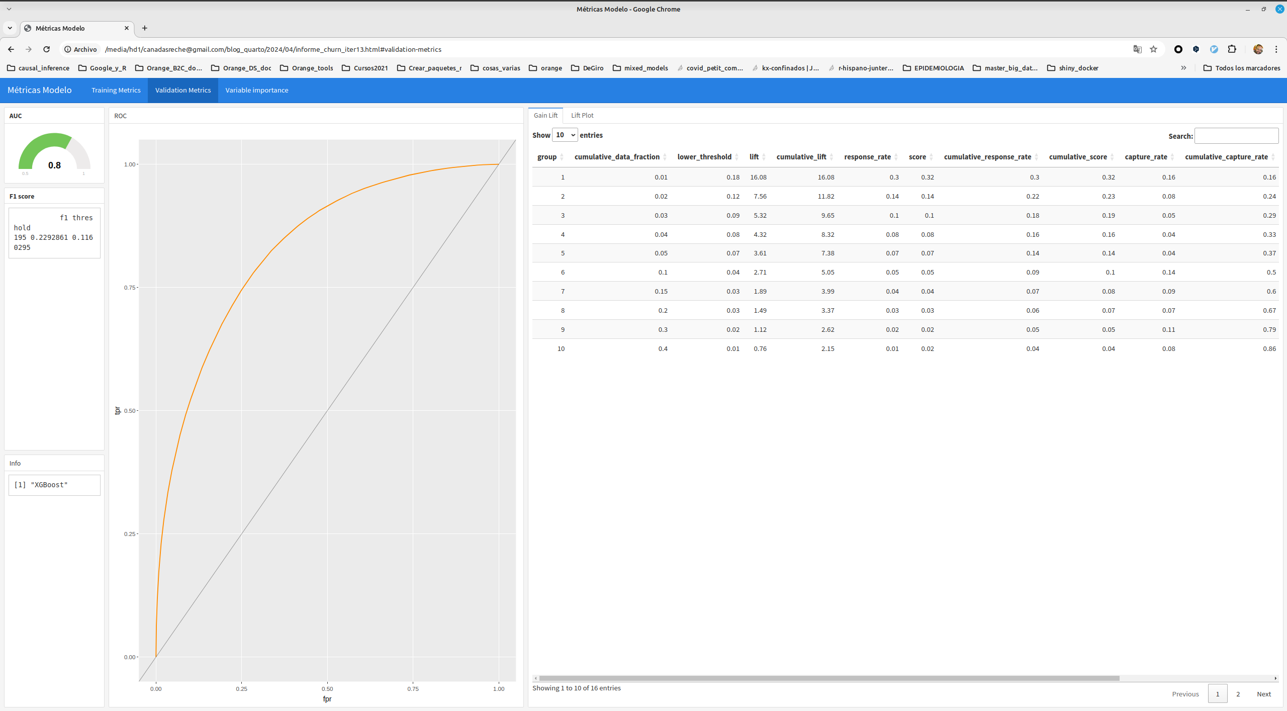
Y esto es todo, de esta forma es como yo en mi día a día guardo un pequeño dashboard de cada modelo, simplemente leyendo la info que h2o ha guardado en el mojo y así estoy seguro de que esas métricas son justo las que corresponden con los datos usados por el modelo.